Correlation

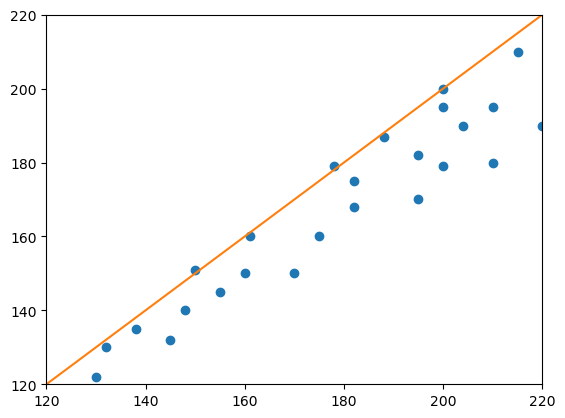
For measuring the relationship between two measurements, we can take Pearson’s definition of a correlation coefficient

The data for the following expriment is taken from Altman & Bland, The Statistician 32, 1983, Fig. 1.

import numpy as np
import matplotlib.pyplot as plt
import pandas as pd
from scipy import stats
import pandas as pd
from sklearn import datasets

# new measurements
measurement_1 = [130, 132, 138, 145, 148, 150, 155, 160, 161, 170, 175, 178, 182, 182, 188, 195, 195, 200, 200, 204, 210, 210, 215, 220, 200]
measurement_2 = [122, 130, 135, 132, 140, 151, 145, 150, 160, 150, 160, 179, 168, 175, 187, 170, 182, 179, 195, 190, 180, 195, 210, 190, 200]

# scatter plot
plt.plot(measurement_1, measurement_2, "o")
plt.plot([120, 220], [120, 220])
plt.axis([120, 220, 120, 220])
plt.show()

Pearson correlation coefficient

We can use the Pearson correlation coefficient to calculate the Pearson correlation coefficient:

\(r_{xy} = \frac{\sum_{i=1}^n (x_i - \mu_x)(y_i - \mu_y)}{\sqrt{(\sum_{i=1}^n(x_i - \mu_x)^2}\sqrt{\sum_{i=1}^n(y_i - \mu_y)^2}}\)

Exercise:

Try to implement this yourself!

Hint: The expressions in the denominator are equivalent to the standard deviations of the data!

…or use the implementation from scipy:

# Determine Pearson's r using scipy
stats.pearsonr(measurement_1, measurement_2)

PearsonRResult(statistic=0.9435300113035255, pvalue=1.6002440484659832e-12)

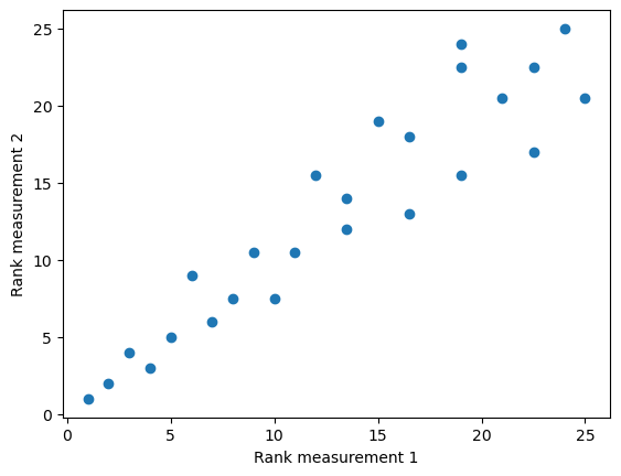
Ranking data

Ranking allows to obtain a non-parametric distribution from our data. In essence, we replace every value with its rank. This iboils down to sorting all the values and replacing the value with its index in the sorted list:

df = pd.DataFrame([measurement_1, measurement_2]).T
df.columns = ['Measurement 1', 'Measurement 2']
df

	Measurement 1	Measurement 2
0	130	122
1	132	130
2	138	135
3	145	132
4	148	140
5	150	151
6	155	145
7	160	150
8	161	160
9	170	150
10	175	160
11	178	179
12	182	168
13	182	175
14	188	187
15	195	170
16	195	182
17	200	179
18	200	195
19	204	190
20	210	180
21	210	195
22	215	210
23	220	190
24	200	200

To rank the data, use, the rankdata functions from scipy.stats

measurement_1_ranked = stats.rankdata(measurement_1)
measurement_2_ranked = stats.rankdata(measurement_2)

fig, ax = plt.subplots()
ax.scatter(measurement_1_ranked, measurement_2_ranked)
ax.set_xlabel('Rank measurement 1')
ax.set_ylabel('Rank measurement 2')

Text(0, 0.5, 'Rank measurement 2')

Spearman rank correlation coefficient

Now, we can use the above-introduced Pearson correlation coefficient - but on the ranked data! This concept is also commonly known as the Spearman correlation coefficient.

Exercise

Calculate the rank correlation coefficient on the ranked data. Use either your above-introduced correlation coefficient calculation or the respective function from scipy.stats

Exercise: Pearson vs. Spearman

Let’s compare both for a few scenarios to highlight their differences. Plot the raw data, the ranked data for the following scenarios and calculate both correlation coefficients

# Scenario 1
x = np.arange(-10,10, 0.5)
x += np.random.random(len(x))*2
y = x**3 + np.random.random(len(x))*10

# Scenario 2
x = np.arange(-10,10, 0.5)
y = np.tanh(x) + np.random.random(len(x))

# Scenario 3
x = np.arange(-10,10, 0.5)
x += np.random.random(len(x))*2
y = -x**3 + np.random.random(len(x))*10