Stardist in Python: Data

This notebook demonstrates the usage of Stardist in Python - one of the most common and powerful tools for nucleus segmetation. Prior to running this notebook, you need to install stardist and tensorflow. It is strongly recommended to create a new environment for this!

conda create -n stardist_tensorflow python=3.9
conda activate stardist_tensorflow

mamba install tensorflow
pip install stardist

Once that is done, you’re good to go:

from __future__ import print_function, unicode_literals, absolute_import, division
import numpy as np
import matplotlib
matplotlib.rcParams["image.interpolation"] = None
import matplotlib.pyplot as plt
%matplotlib inline
%config InlineBackend.figure_format = 'retina'

from glob import glob
from tqdm import tqdm
from tifffile import imread
from csbdeep.utils import Path, download_and_extract_zip_file

from stardist import fill_label_holes, relabel_image_stardist, random_label_cmap
from stardist.matching import matching_dataset

np.random.seed(42)
lbl_cmap = random_label_cmap()

C:\Users\johamuel\AppData\Local\Temp\ipykernel_19440\3639107371.py:4: MatplotlibDeprecationWarning: Support for setting an rcParam that expects a str value to a non-str value is deprecated since 3.5 and support will be removed two minor releases later.
  matplotlib.rcParams["image.interpolation"] = None

Data

This notebook demonstrates how the training data for StarDist should look like and whether the annotated objects can be appropriately described by star-convex polygons.

The training data that needs to be provided for StarDist consists of corresponding pairs of raw images and pixelwise annotated ground truth images (masks), where every pixel has a unique integer value indicating the object id (or 0 for background).

For this demo we will download the file dsb2018.zip that contains the respective train and test images with associated ground truth labels as used in our paper. They are a subset of the stage1_train images from the Kaggle 2018 Data Science Bowl, which are available in full from the Broad Bioimage Benchmark Collection.

download_and_extract_zip_file(
    url       = 'https://github.com/stardist/stardist/releases/download/0.1.0/dsb2018.zip',
    targetdir = 'data',
    verbose   = 1,
)

Files missing, downloading... extracting... done.

X = sorted(glob('data/dsb2018/train/images/*.tif'))
Y = sorted(glob('data/dsb2018/train/masks/*.tif'))
assert all(Path(x).name==Path(y).name for x,y in zip(X,Y))

Load only a small subset

X, Y = X[:10], Y[:10]

X = list(map(imread,X))
Y = list(map(imread,Y))

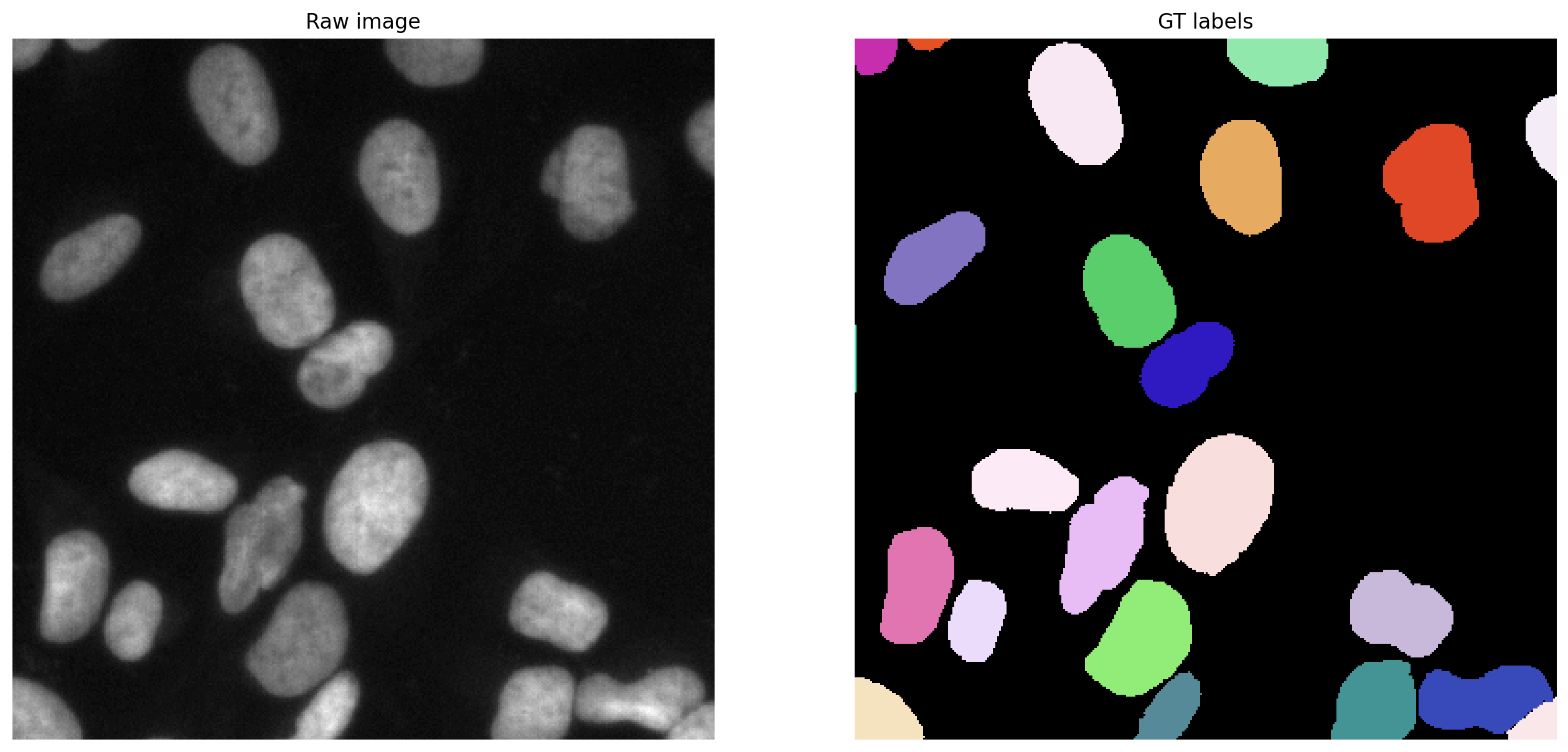
Example image

i = min(4, len(X)-1)
img, lbl = X[i], fill_label_holes(Y[i])
assert img.ndim in (2,3)
img = img if img.ndim==2 else img[...,:3]
# assumed axes ordering of img and lbl is: YX(C)

plt.figure(figsize=(16,10))
plt.subplot(121); plt.imshow(img,cmap='gray');   plt.axis('off'); plt.title('Raw image')
plt.subplot(122); plt.imshow(lbl,cmap=lbl_cmap); plt.axis('off'); plt.title('GT labels')
None;

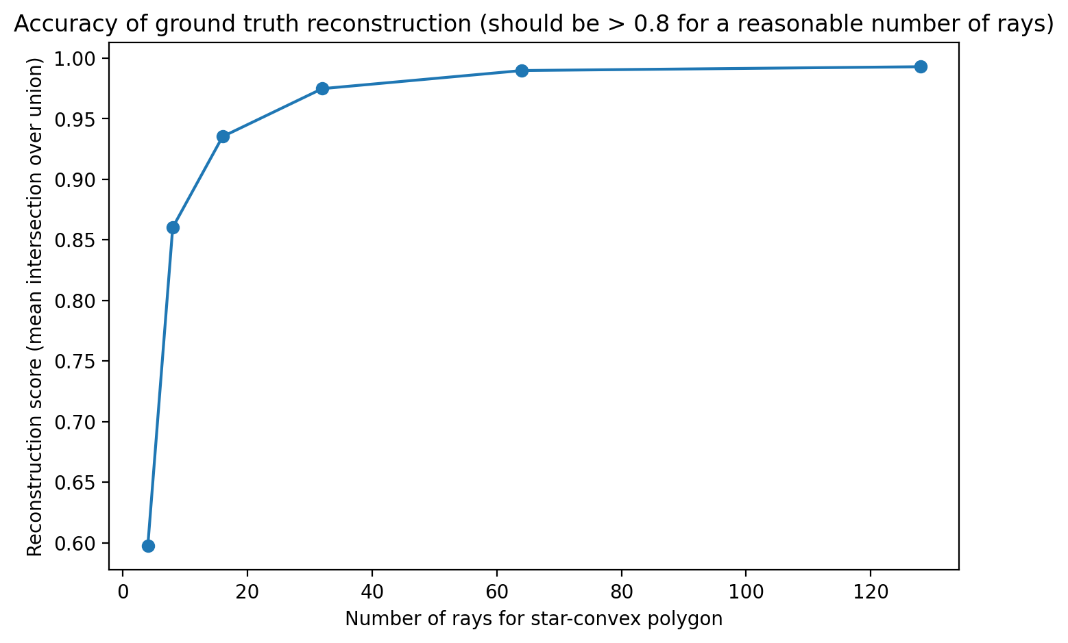
Fitting ground-truth labels with star-convex polygons

As shown in the lecture, the key idea of Stardist is to approximate the nucleus shape by casting rays outwards from a detected center and measureing the probability that the encountered pixels along the way are part of a given nucleus. This brings a key choice with it: The more rays are used to approximate shape, the closer the “true” shape is approximated, but the computation overhead gets larger, too.

We can measure how well the “true” (measured from the annotation) area of the cell is reflected depending on how many rays were used:

n_rays = [2**i for i in range(2,8)]
scores = []
for r in tqdm(n_rays):
    Y_reconstructed = [relabel_image_stardist(lbl, n_rays=r) for lbl in Y]
    mean_iou = matching_dataset(Y, Y_reconstructed, thresh=0, show_progress=False).mean_true_score
    scores.append(mean_iou)

100%|███████████████████████████████████████████████████████████████████████████| 6/6 [00:15<00:00,  2.53s/it]

plt.figure(figsize=(8,5))
plt.plot(n_rays, scores, 'o-')
plt.xlabel('Number of rays for star-convex polygon')
plt.ylabel('Reconstruction score (mean intersection over union)')
plt.title("Accuracy of ground truth reconstruction (should be > 0.8 for a reasonable number of rays)")
None;

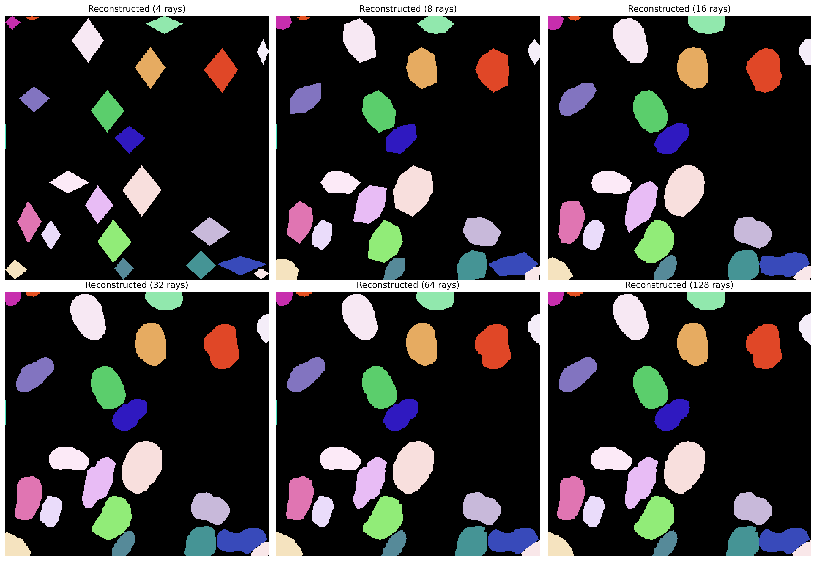
Example image reconstructed with various number of rays

fig, ax = plt.subplots(2,3, figsize=(16,11))
for a,r in zip(ax.flat,n_rays):
    a.imshow(relabel_image_stardist(lbl, n_rays=r), cmap=lbl_cmap)
    a.set_title('Reconstructed (%d rays)' % r)
    a.axis('off')
plt.tight_layout();