Descriptive statistics of labeled images
Contents
Descriptive statistics of labeled images#
Using pandas and numpy, we can do basic descriptive statistics. Before we start, we derive some measurements from an labeled image.
import pandas as pd
import numpy as np
from skimage.io import imread, imshow
from napari_segment_blobs_and_things_with_membranes import gauss_otsu_labeling
from skimage.measure import regionprops_table
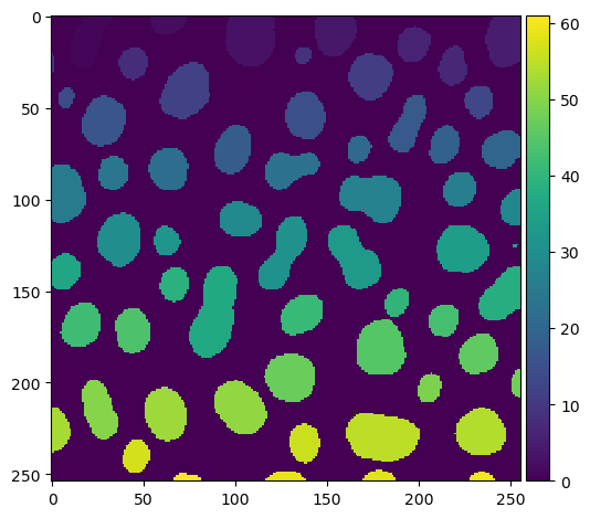
We load the image using scikit-image’s imread and segment it using Gauss-Otsu-Labeling.
image = imread('../../data/blobs.tif')
labels = np.asarray(gauss_otsu_labeling(image))
imshow(labels)
C:\Users\Marcelo_Researcher\anaconda3\envs\devbio-napari-env\lib\site-packages\skimage\io\_plugins\matplotlib_plugin.py:150: UserWarning: Low image data range; displaying image with stretched contrast.
  lo, hi, cmap = _get_display_range(image)
<matplotlib.image.AxesImage at 0x1f69e39eac0>
From the labeled image we can derive descriptive intensity, size and shape statistics using scikit-image’s regionprops_table.
For post-processing the measurements, we turn them into a pandas Dataframe.
table = regionprops_table(labels, image, properties=['area', 'minor_axis_length', 'major_axis_length', 'eccentricity', 'feret_diameter_max'])
data_frame = pd.DataFrame(table)
data_frame
| area | minor_axis_length | major_axis_length | eccentricity | feret_diameter_max | |
|---|---|---|---|---|---|
| 0 | 422 | 16.488550 | 34.566789 | 0.878900 | 35.227830 |
| 1 | 182 | 11.736074 | 20.802697 | 0.825665 | 21.377558 |
| 2 | 661 | 28.409502 | 30.208433 | 0.339934 | 32.756679 |
| 3 | 437 | 23.143996 | 24.606130 | 0.339576 | 26.925824 |
| 4 | 476 | 19.852882 | 31.075106 | 0.769317 | 31.384710 |
| ... | ... | ... | ... | ... | ... |
| 56 | 211 | 14.522762 | 18.489138 | 0.618893 | 18.973666 |
| 57 | 78 | 6.028638 | 17.579799 | 0.939361 | 18.027756 |
| 58 | 86 | 5.426871 | 21.261427 | 0.966876 | 22.000000 |
| 59 | 51 | 5.032414 | 13.742079 | 0.930534 | 14.035669 |
| 60 | 46 | 3.803982 | 15.948714 | 0.971139 | 15.033296 |
61 rows × 5 columns
You can take a column out of the DataFrame. In this context it works like a Python dictionary.
data_frame["area"]
0     422
1     182
2     661
3     437
4     476
     ...
56    211
57     78
58     86
59     51
60     46
Name: area, Length: 61, dtype: int32
Even though this data structure appears more than just a vector, numpy is capable of applying basic descriptive statistics functions:
np.mean(data_frame["area"])
358.42622950819674
np.min(data_frame["area"])
5
np.max(data_frame["area"])
899
Individual cells of the DataFrame can be accessed like this:
data_frame.loc[0, "area"]
422
Summary statistics with Pandas#
Pandas also allows you to visualize summary statistics of measurement using the describe() function.
data_frame.describe()
| area | minor_axis_length | major_axis_length | eccentricity | feret_diameter_max | |
|---|---|---|---|---|---|
| count | 61.000000 | 61.000000 | 61.000000 | 61.000000 | 61.000000 |
| mean | 358.426230 | 17.127032 | 24.796851 | 0.657902 | 25.323368 |
| std | 210.446942 | 6.587838 | 9.074265 | 0.189669 | 8.732456 |
| min | 5.000000 | 1.788854 | 3.098387 | 0.312788 | 3.162278 |
| 25% | 205.000000 | 14.319400 | 18.630719 | 0.503830 | 19.313208 |
| 50% | 375.000000 | 17.523565 | 23.768981 | 0.645844 | 24.698178 |
| 75% | 503.000000 | 21.753901 | 30.208433 | 0.825665 | 31.384710 |
| max | 899.000000 | 28.409502 | 54.500296 | 0.984887 | 52.201533 |
Correlation matrix#
If you want to learn which parameters are correlated with other parameters, you can visualize that using pandas’s corr().
data_frame.corr()
| area | minor_axis_length | major_axis_length | eccentricity | feret_diameter_max | |
|---|---|---|---|---|---|
| area | 1.000000 | 0.890649 | 0.895282 | -0.192147 | 0.916652 |
| minor_axis_length | 0.890649 | 1.000000 | 0.664507 | -0.566486 | 0.716706 |
| major_axis_length | 0.895282 | 0.664507 | 1.000000 | 0.168454 | 0.995196 |
| eccentricity | -0.192147 | -0.566486 | 0.168454 | 1.000000 | 0.103529 |
| feret_diameter_max | 0.916652 | 0.716706 | 0.995196 | 0.103529 | 1.000000 |