Stardist in Python: Training
Contents
Stardist in Python: Training#
This notebook will demonstrate how to train your own stardist model based on the data you should have downloaded in the [previous notebook].(./01_Stardist2d_in_python_getting_data.ipynb)
from __future__ import print_function, unicode_literals, absolute_import, division
import sys
import numpy as np
import matplotlib
matplotlib.rcParams["image.interpolation"] = None
import matplotlib.pyplot as plt
%matplotlib inline
%config InlineBackend.figure_format = 'retina'

from glob import glob
from tqdm import tqdm
from tifffile import imread
from csbdeep.utils import Path, normalize

from skimage import transform

from stardist import fill_label_holes, random_label_cmap, calculate_extents, gputools_available
from stardist.matching import matching, matching_dataset
from stardist.models import Config2D, StarDist2D, StarDistData2D

np.random.seed(42)
lbl_cmap = random_label_cmap()
1108461538.py (5): Support for setting an rcParam that expects a str value to a non-str value is deprecated since 3.5 and support will be removed two minor releases later.
Data#
X = sorted(glob('data/dsb2018/train/images/*.tif'))
Y = sorted(glob('data/dsb2018/train/masks/*.tif'))
assert all(Path(x).name==Path(y).name for x,y in zip(X,Y))
X = list(map(imread,X))
Y = list(map(imread,Y))
n_channel = 1 if X[0].ndim == 2 else X[0].shape[-1]
Normalize images and fill small label holes.
axis_norm = (0,1)   # normalize channels independently
# axis_norm = (0,1,2) # normalize channels jointly
if n_channel > 1:
    print("Normalizing image channels %s." % ('jointly' if axis_norm is None or 2 in axis_norm else 'independently'))
    sys.stdout.flush()

X = [normalize(x,1,99.8,axis=axis_norm) for x in tqdm(X)]
Y = [fill_label_holes(y) for y in tqdm(Y)]
100%|██████████████████████████████████████████████████████████████████████| 447/447 [00:00<00:00, 452.66it/s]
100%|██████████████████████████████████████████████████████████████████████| 447/447 [00:01<00:00, 238.41it/s]
Split into train and validation datasets.
assert len(X) > 1, "not enough training data"
rng = np.random.RandomState(42)
ind = rng.permutation(len(X))
n_val = max(1, int(round(0.15 * len(ind))))
ind_train, ind_val = ind[:-n_val], ind[-n_val:]
X_val, Y_val = [X[i] for i in ind_val]  , [Y[i] for i in ind_val]
X_trn, Y_trn = [X[i] for i in ind_train], [Y[i] for i in ind_train]
print('number of images: %3d' % len(X))
print('- training:       %3d' % len(X_trn))
print('- validation:     %3d' % len(X_val))
number of images: 447
- training:       380
- validation:      67
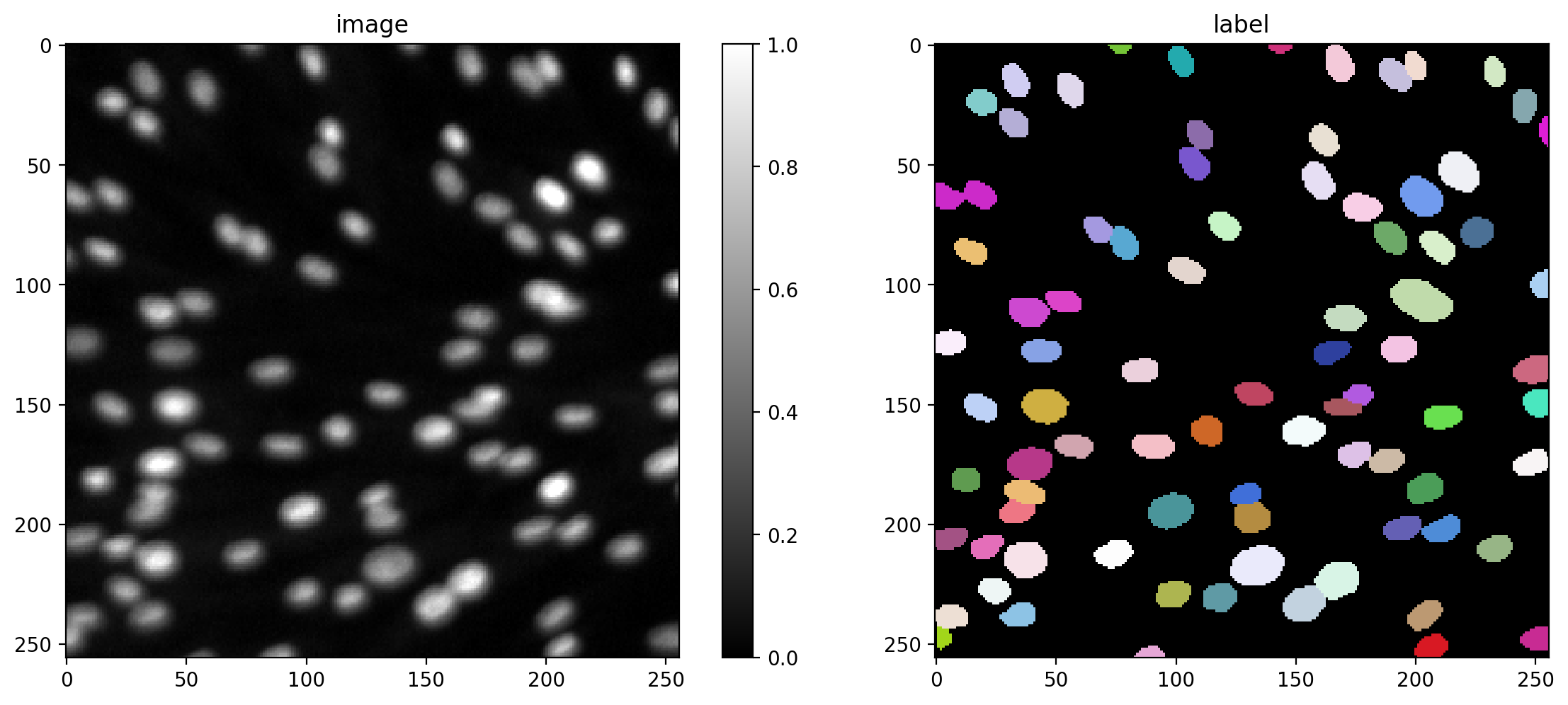
Training data consists of pairs of input image and label instances.
def plot_img_label(img, lbl, img_title="image", lbl_title="label", **kwargs):
    fig, (ai,al) = plt.subplots(1,2, figsize=(12,5), gridspec_kw=dict(width_ratios=(1.25,1)))
    im = ai.imshow(img, cmap='gray', clim=(0,1))
    ai.set_title(img_title)
    fig.colorbar(im, ax=ai)
    al.imshow(lbl, cmap=lbl_cmap)
    al.set_title(lbl_title)
    plt.tight_layout()
i = min(9, len(X)-1)
img, lbl = X[i], Y[i]
assert img.ndim in (2,3)
img = img if (img.ndim==2 or img.shape[-1]==3) else img[...,0]
plot_img_label(img,lbl)
None;
Configuration#
A StarDist2D model is specified via a Config2D object.
print(Config2D.__doc__)
Configuration for a :class:`StarDist2D` model.

    Parameters
    ----------
    axes : str or None
        Axes of the input images.
    n_rays : int
        Number of radial directions for the star-convex polygon.
        Recommended to use a power of 2 (default: 32).
    n_channel_in : int
        Number of channels of given input image (default: 1).
    grid : (int,int)
        Subsampling factors (must be powers of 2) for each of the axes.
        Model will predict on a subsampled grid for increased efficiency and larger field of view.
    n_classes : None or int
        Number of object classes to use for multi-class predection (use None to disable)
    backbone : str
        Name of the neural network architecture to be used as backbone.
    kwargs : dict
        Overwrite (or add) configuration attributes (see below).


    Attributes
    ----------
    unet_n_depth : int
        Number of U-Net resolution levels (down/up-sampling layers).
    unet_kernel_size : (int,int)
        Convolution kernel size for all (U-Net) convolution layers.
    unet_n_filter_base : int
        Number of convolution kernels (feature channels) for first U-Net layer.
        Doubled after each down-sampling layer.
    unet_pool : (int,int)
        Maxpooling size for all (U-Net) convolution layers.
    net_conv_after_unet : int
        Number of filters of the extra convolution layer after U-Net (0 to disable).
    unet_* : *
        Additional parameters for U-net backbone.
    train_shape_completion : bool
        Train model to predict complete shapes for partially visible objects at image boundary.
    train_completion_crop : int
        If 'train_shape_completion' is set to True, specify number of pixels to crop at boundary of training patches.
        Should be chosen based on (largest) object sizes.
    train_patch_size : (int,int)
        Size of patches to be cropped from provided training images.
    train_background_reg : float
        Regularizer to encourage distance predictions on background regions to be 0.
    train_foreground_only : float
        Fraction (0..1) of patches that will only be sampled from regions that contain foreground pixels.
    train_sample_cache : bool
        Activate caching of valid patch regions for all training images (disable to save memory for large datasets)
    train_dist_loss : str
        Training loss for star-convex polygon distances ('mse' or 'mae').
    train_loss_weights : tuple of float
        Weights for losses relating to (probability, distance)
    train_epochs : int
        Number of training epochs.
    train_steps_per_epoch : int
        Number of parameter update steps per epoch.
    train_learning_rate : float
        Learning rate for training.
    train_batch_size : int
        Batch size for training.
    train_n_val_patches : int
        Number of patches to be extracted from validation images (``None`` = one patch per image).
    train_tensorboard : bool
        Enable TensorBoard for monitoring training progress.
    train_reduce_lr : dict
        Parameter :class:`dict` of ReduceLROnPlateau_ callback; set to ``None`` to disable.
    use_gpu : bool
        Indicate that the data generator should use OpenCL to do computations on the GPU.

        .. _ReduceLROnPlateau: https://keras.io/api/callbacks/reduce_lr_on_plateau/
Before actually doing the training, we need to set some parameters. Predominantly these parameters are
Number of rays: See previous notebook
Use the graphics card for training: This is disabled by default and will not work on PCs without an NVidia graphics card. It may be possible to enable this feature on your PC by downloading cudatoolkit - no guarantuee given, though.
grid: The size of the image may be too large for your memory to handle during training - thus it is common to split the image into tiles and process these tiles separately.
# 32 is a good default choice (see 1_data.ipynb)
n_rays = 32

# Use OpenCL-based computations for data generator during training (requires 'gputools')
use_gpu = False and gputools_available()

# Predict on subsampled grid for increased efficiency and larger field of view
grid = (2,2)

conf = Config2D (
    n_rays       = n_rays,
    grid         = grid,
    use_gpu      = use_gpu,
    n_channel_in = n_channel,
)
print(conf)
vars(conf)
Config2D(n_dim=2, axes='YXC', n_channel_in=1, n_channel_out=33, train_checkpoint='weights_best.h5', train_checkpoint_last='weights_last.h5', train_checkpoint_epoch='weights_now.h5', n_rays=32, grid=(2, 2), backbone='unet', n_classes=None, unet_n_depth=3, unet_kernel_size=(3, 3), unet_n_filter_base=32, unet_n_conv_per_depth=2, unet_pool=(2, 2), unet_activation='relu', unet_last_activation='relu', unet_batch_norm=False, unet_dropout=0.0, unet_prefix='', net_conv_after_unet=128, net_input_shape=(None, None, 1), net_mask_shape=(None, None, 1), train_shape_completion=False, train_completion_crop=32, train_patch_size=(256, 256), train_background_reg=0.0001, train_foreground_only=0.9, train_sample_cache=True, train_dist_loss='mae', train_loss_weights=(1, 0.2), train_class_weights=(1, 1), train_epochs=400, train_steps_per_epoch=100, train_learning_rate=0.0003, train_batch_size=4, train_n_val_patches=None, train_tensorboard=True, train_reduce_lr={'factor': 0.5, 'patience': 40, 'min_delta': 0}, use_gpu=False)
{'n_dim': 2,
 'axes': 'YXC',
 'n_channel_in': 1,
 'n_channel_out': 33,
 'train_checkpoint': 'weights_best.h5',
 'train_checkpoint_last': 'weights_last.h5',
 'train_checkpoint_epoch': 'weights_now.h5',
 'n_rays': 32,
 'grid': (2, 2),
 'backbone': 'unet',
 'n_classes': None,
 'unet_n_depth': 3,
 'unet_kernel_size': (3, 3),
 'unet_n_filter_base': 32,
 'unet_n_conv_per_depth': 2,
 'unet_pool': (2, 2),
 'unet_activation': 'relu',
 'unet_last_activation': 'relu',
 'unet_batch_norm': False,
 'unet_dropout': 0.0,
 'unet_prefix': '',
 'net_conv_after_unet': 128,
 'net_input_shape': (None, None, 1),
 'net_mask_shape': (None, None, 1),
 'train_shape_completion': False,
 'train_completion_crop': 32,
 'train_patch_size': (256, 256),
 'train_background_reg': 0.0001,
 'train_foreground_only': 0.9,
 'train_sample_cache': True,
 'train_dist_loss': 'mae',
 'train_loss_weights': (1, 0.2),
 'train_class_weights': (1, 1),
 'train_epochs': 400,
 'train_steps_per_epoch': 100,
 'train_learning_rate': 0.0003,
 'train_batch_size': 4,
 'train_n_val_patches': None,
 'train_tensorboard': True,
 'train_reduce_lr': {'factor': 0.5, 'patience': 40, 'min_delta': 0},
 'use_gpu': False}
if use_gpu:
    from csbdeep.utils.tf import limit_gpu_memory
    # adjust as necessary: limit GPU memory to be used by TensorFlow to leave some to OpenCL-based computations
    limit_gpu_memory(0.8)
    # alternatively, try this:
    # limit_gpu_memory(None, allow_growth=True)
Note: The trained StarDist2D model will not predict completed shapes for partially visible objects at the image boundary if train_shape_completion=False (which is the default option).
model = StarDist2D(conf, name='stardist', basedir='models')
Loading thresholds from 'thresholds.json'.
Using default values: prob_thresh=0.24019, nms_thresh=0.3.
Check if the neural network has a large enough field of view to see up to the boundary of most objects.
median_size = calculate_extents(list(Y), np.median)
fov = np.array(model._axes_tile_overlap('YX'))
print(f"median object size:      {median_size}")
print(f"network field of view :  {fov}")
if any(median_size > fov):
    print("WARNING: median object size larger than field of view of the neural network.")
1/1 [==============================] - 0s 182ms/step
1/1 [==============================] - 0s 61ms/step
median object size:      [17.5 18. ]
network field of view :  [94 94]
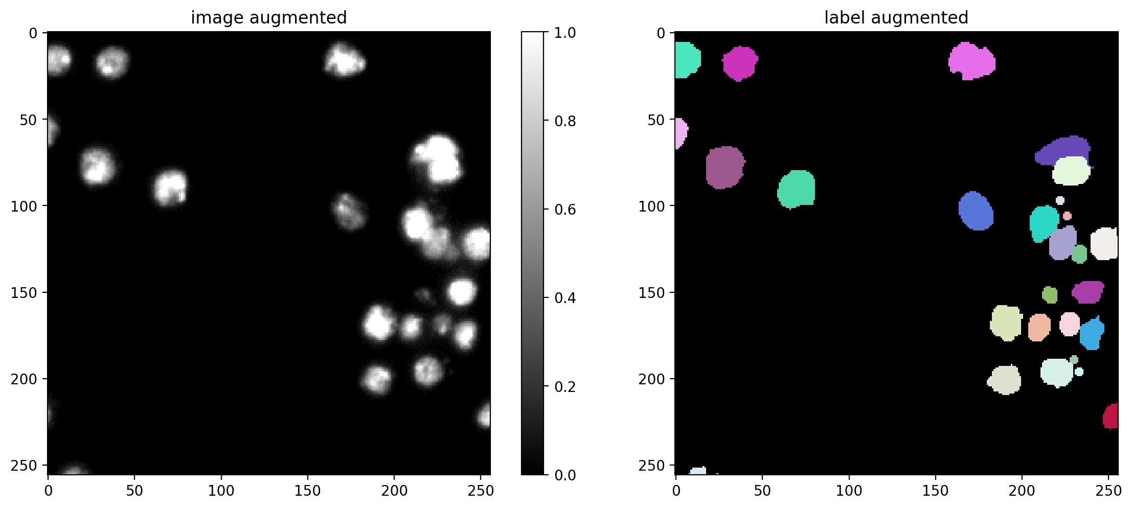
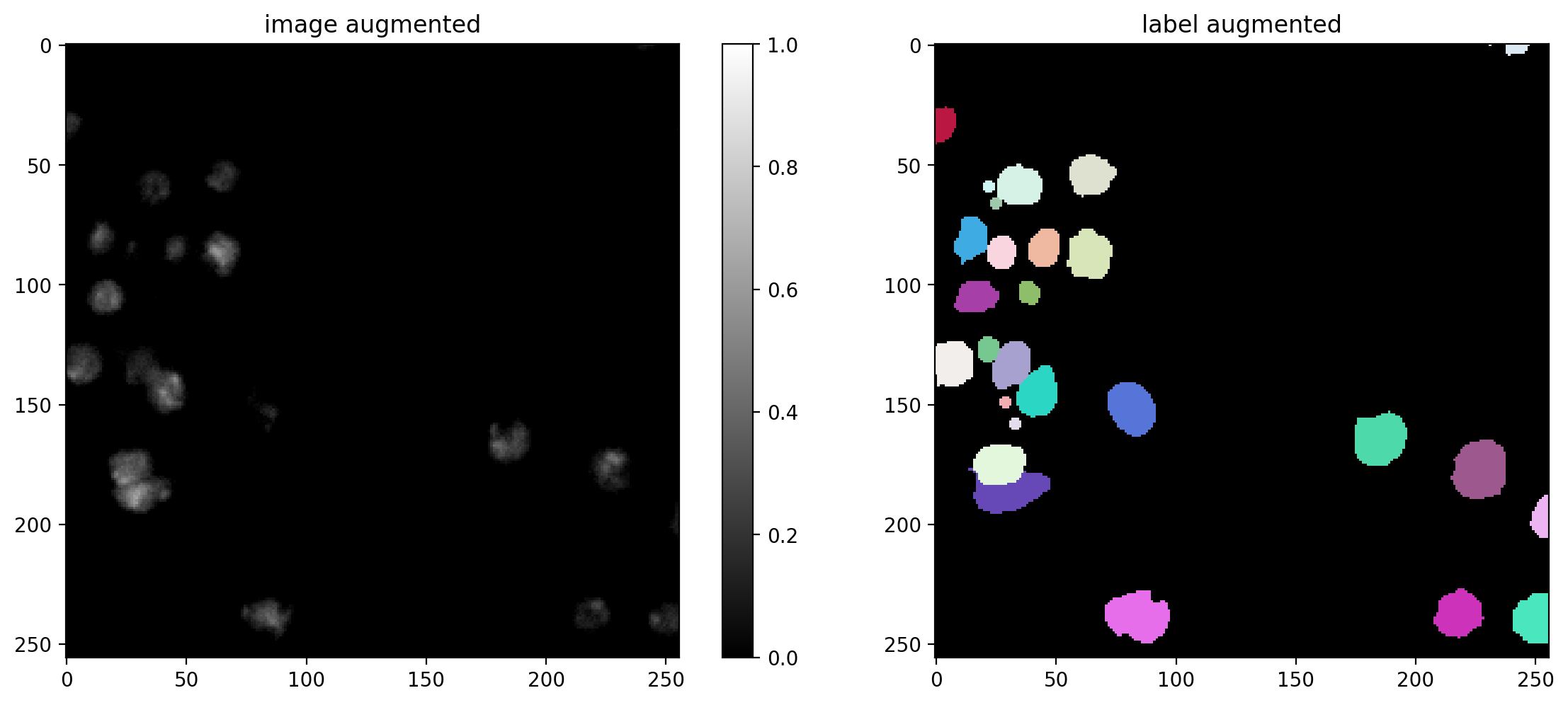
Data Augmentation#
You can define a function/callable that applies augmentation to each batch of the data generator.
We here use an augmenter that applies random rotations, flips, and intensity changes, which are typically sensible for (2D) microscopy images (but you can disable augmentation by setting augmenter = None).
def random_fliprot(img, mask):
    assert img.ndim >= mask.ndim
    axes = tuple(range(mask.ndim))
    perm = tuple(np.random.permutation(axes))
    img = img.transpose(perm + tuple(range(mask.ndim, img.ndim)))
    mask = mask.transpose(perm)
    for ax in axes:
        if np.random.rand() > 0.5:
            img = np.flip(img, axis=ax)
            mask = np.flip(mask, axis=ax)
    return img, mask

def random_intensity_change(img):
    img = img*np.random.uniform(0.6,2) + np.random.uniform(-0.2,0.2)
    return img


def augmenter(x, y):
    """Augmentation of a single input/label image pair.
    x is an input image
    y is the corresponding ground-truth label image
    """
    x, y = random_fliprot(x, y)
    x = random_intensity_change(x)
    # add some gaussian noise
    sig = 0.02*np.random.uniform(0,1)
    x = x + sig*np.random.normal(0,1,x.shape)
    return x, y
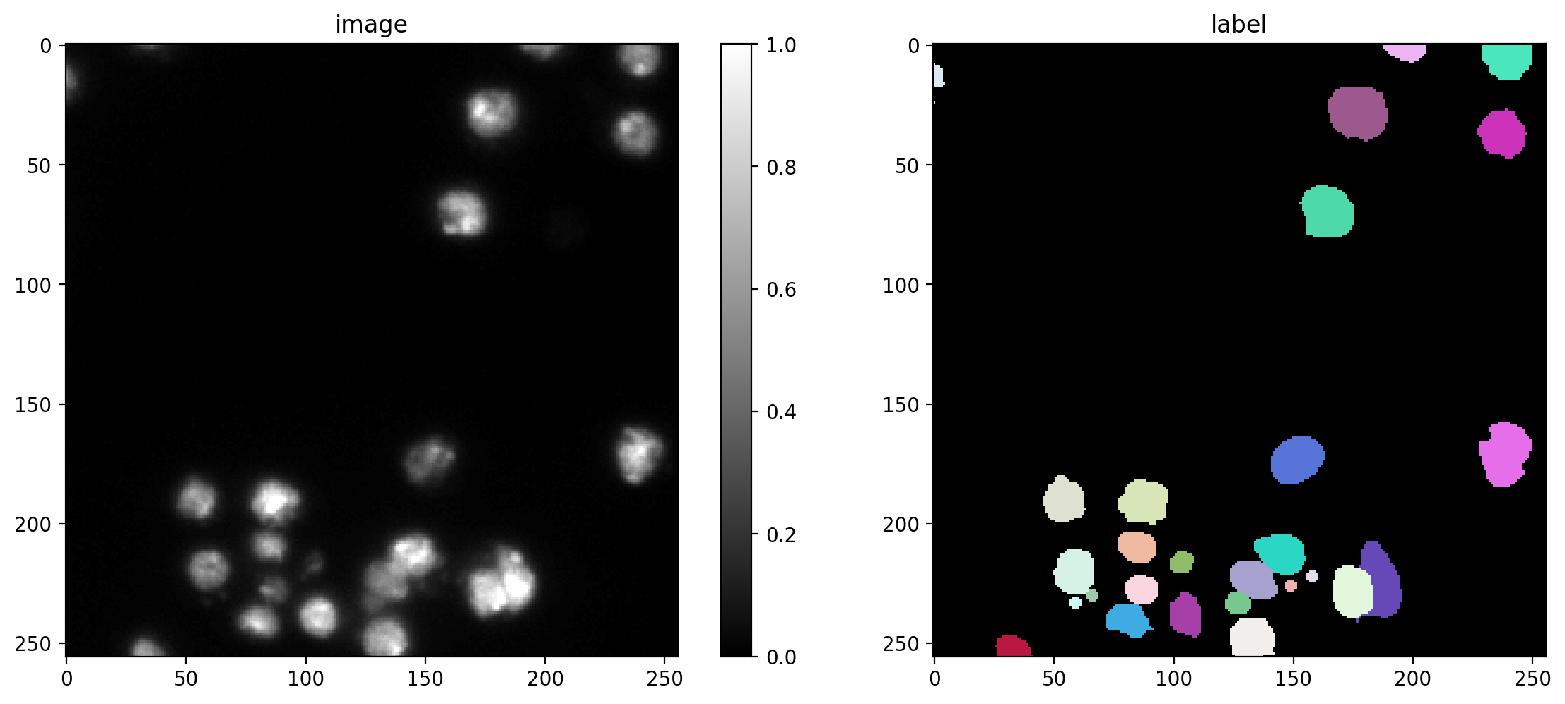
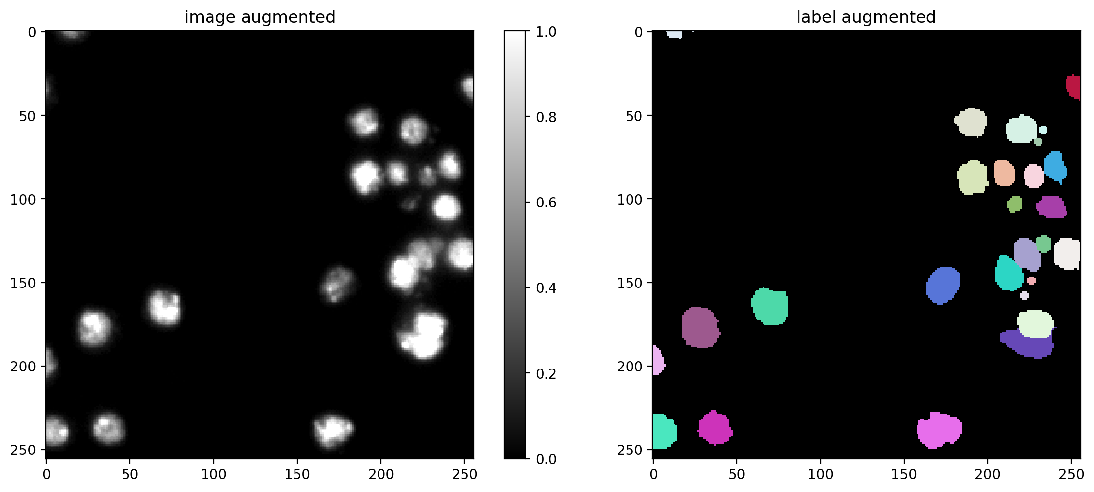
# plot some augmented examples
img, lbl = X[0],Y[0]
plot_img_label(img, lbl)
for _ in range(3):
    img_aug, lbl_aug = augmenter(img,lbl)
    plot_img_label(img_aug, lbl_aug, img_title="image augmented", lbl_title="label augmented")
Training#
We recommend to monitor the progress during training with TensorBoard. You can start it in the shell from the current working directory like this:
$ tensorboard --logdir=.
Then connect to http://localhost:6006/ with your browser.
quick_demo = True

if quick_demo:
    print (
        "NOTE: This is only for a quick demonstration!\n"
        "      Please set the variable 'quick_demo = False' for proper (long) training.",
        file=sys.stderr, flush=True
    )
    model.train(X_trn, Y_trn, validation_data=(X_val,Y_val), augmenter=augmenter,
                epochs=2, steps_per_epoch=10)

    print("====> Stopping training and loading previously trained demo model from disk.", file=sys.stderr, flush=True)
    model = StarDist2D.from_pretrained('2D_demo')
else:
    model.train(X_trn, Y_trn, validation_data=(X_val,Y_val), augmenter=augmenter)
None;
NOTE: This is only for a quick demonstration!
      Please set the variable 'quick_demo = False' for proper (long) training.
Epoch 1/2
3/3 [==============================] - 0s 45ms/steploss: 1.7712 - prob_loss: 0.3109 - dist_loss: 7.3018 - prob_kld: 0.2339 - dist_relevant_mae: 7.3011 - dist_relevant_mse: 111.6556 - dist_dist_iou_metric: 0.
10/10 [==============================] - 10s 1s/step - loss: 1.7712 - prob_loss: 0.3109 - dist_loss: 7.3018 - prob_kld: 0.2339 - dist_relevant_mae: 7.3011 - dist_relevant_mse: 111.6556 - dist_dist_iou_metric: 0.3070 - val_loss: 1.8127 - val_prob_loss: 0.2679 - val_dist_loss: 7.7241 - val_prob_kld: 0.1960 - val_dist_relevant_mae: 7.7235 - val_dist_relevant_mse: 135.9931 - val_dist_dist_iou_metric: 0.2631 - lr: 3.0000e-04
Epoch 2/2
3/3 [==============================] - 0s 40ms/steploss: 1.9356 - prob_loss: 0.3372 - dist_loss: 7.9920 - prob_kld: 0.2581 - dist_relevant_mae: 7.9912 - dist_relevant_mse: 129.1611 - dist_dist_iou_metric: 0.
10/10 [==============================] - 10s 1s/step - loss: 1.9356 - prob_loss: 0.3372 - dist_loss: 7.9920 - prob_kld: 0.2581 - dist_relevant_mae: 7.9912 - dist_relevant_mse: 129.1611 - dist_dist_iou_metric: 0.3146 - val_loss: 1.8624 - val_prob_loss: 0.3237 - val_dist_loss: 7.6934 - val_prob_kld: 0.2518 - val_dist_relevant_mae: 7.6928 - val_dist_relevant_mse: 135.1480 - val_dist_dist_iou_metric: 0.2563 - lr: 3.0000e-04

Loading network weights from 'weights_best.h5'.
====> Stopping training and loading previously trained demo model from disk.
Found model '2D_demo' for 'StarDist2D'.
Loading network weights from 'weights_best.h5'.
Loading thresholds from 'thresholds.json'.
Using default values: prob_thresh=0.486166, nms_thresh=0.5.
Threshold optimization#
While the default values for the probability and non-maximum suppression thresholds already yield good results in many cases, we still recommend to adapt the thresholds to your data. The optimized threshold values are saved to disk and will be automatically loaded with the model.
if quick_demo:
    model.optimize_thresholds(X_val[:2], Y_val[:2])
else:
    model.optimize_thresholds(X_val, Y_val)
1/1 [==============================] - 0s 195ms/step
1/1 [==============================] - 0s 83ms/step
NMS threshold = 0.3:  75%|███████████████████████████         | 15/20 [00:01<00:00, 10.23it/s, 0.511 -> 0.700]
NMS threshold = 0.4:  75%|███████████████████████████         | 15/20 [00:01<00:00,  9.82it/s, 0.511 -> 0.688]
NMS threshold = 0.5:  75%|███████████████████████████         | 15/20 [00:01<00:00, 10.23it/s, 0.511 -> 0.688]
Using optimized values: prob_thresh=0.508553, nms_thresh=0.3.
Evaluation and Detection Performance#
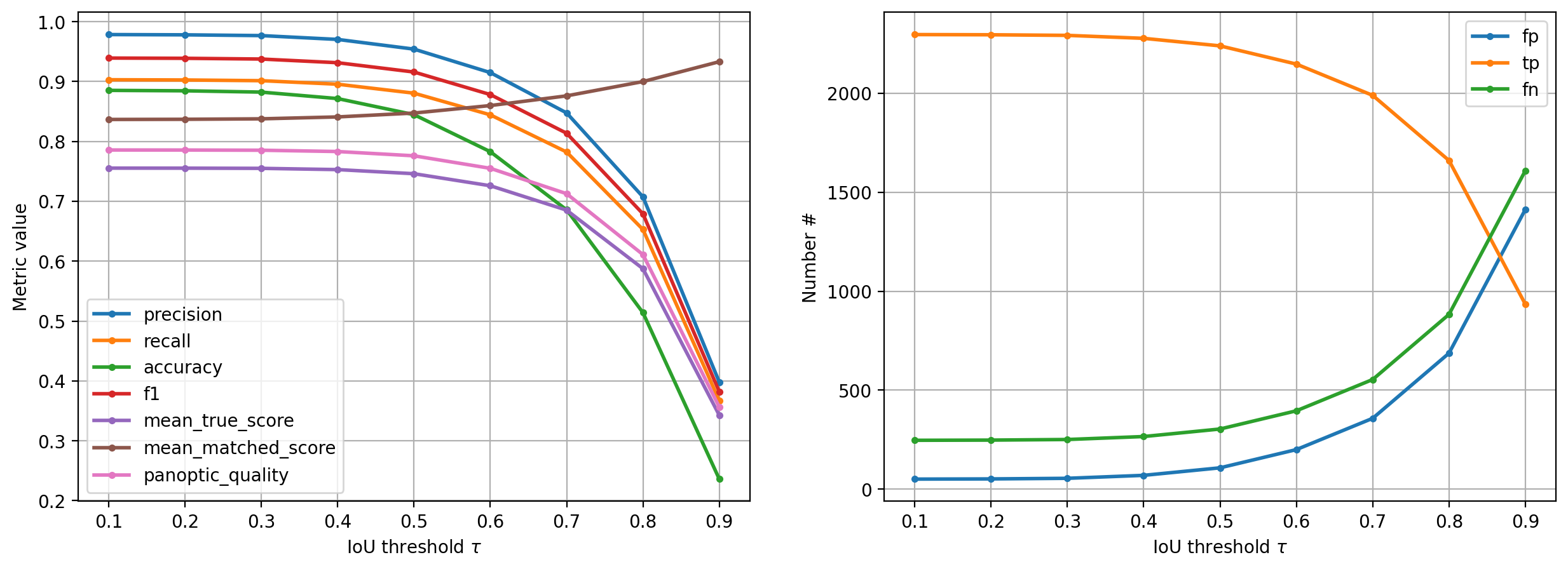
Besides the losses and metrics during training, we can also quantitatively evaluate the actual detection/segmentation performance on the validation data by considering objects in the ground truth to be correctly matched if there are predicted objects with overlap (here intersection over union (IoU)) beyond a chosen IoU threshold \(\tau\).
The corresponding matching statistics (average overlap, accuracy, recall, precision, etc.) are typically of greater practical relevance than the losses/metrics computed during training (but harder to formulate as a loss function). The value of \(\tau\) can be between 0 (even slightly overlapping objects count as correctly predicted) and 1 (only pixel-perfectly overlapping objects count) and which \(\tau\) to use depends on the needed segmentation precision/application.
Please see help(matching) for definitions of the abbreviations used in the evaluation below and see the Wikipedia page on Sensitivity and specificity for further details.
# help(matching)
First predict the labels for all validation images:
Y_val_pred = [model.predict_instances(x, n_tiles=model._guess_n_tiles(x), show_tile_progress=False)[0]
              for x in tqdm(X_val)]
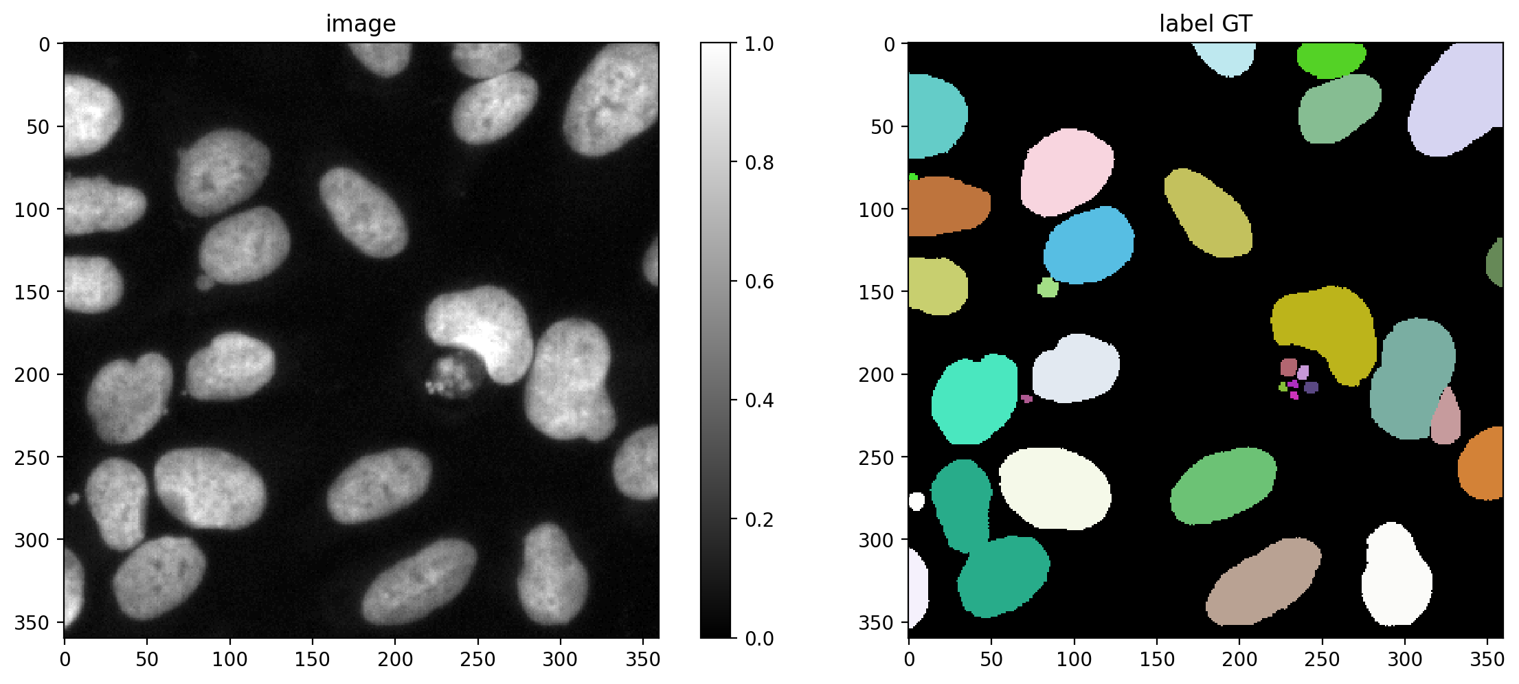
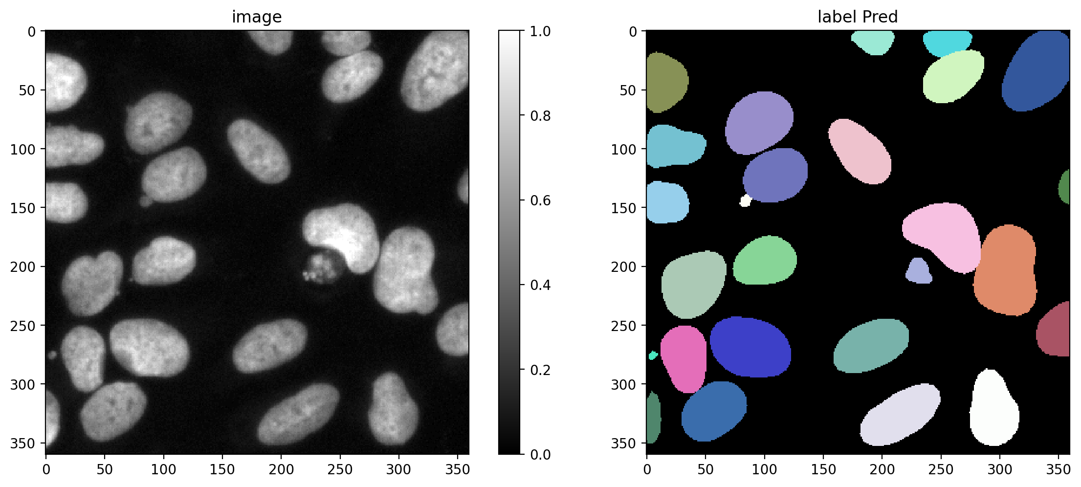
Plot a GT/prediction example
plot_img_label(X_val[0],Y_val[0], lbl_title="label GT")
plot_img_label(X_val[0],Y_val_pred[0], lbl_title="label Pred")
Choose several IoU thresholds \(\tau\) that might be of interest and for each compute matching statistics for the validation data.
taus = [0.1, 0.2, 0.3, 0.4, 0.5, 0.6, 0.7, 0.8, 0.9]
stats = [matching_dataset(Y_val, Y_val_pred, thresh=t, show_progress=False) for t in tqdm(taus)]
100%|███████████████████████████████████████████████████████████████████████████| 9/9 [00:02<00:00, 3.82it/s]
Example: Print all available matching statistics for \(\tau=0.5\)
stats[taus.index(0.5)]
DatasetMatching(criterion='iou', thresh=0.5, fp=108, tp=2239, fn=304, precision=0.953983809118023, recall=0.8804561541486433, accuracy=0.8445869483213881, f1=0.9157464212678936, n_true=2543, n_pred=2347, mean_true_score=0.7459801213740365, mean_matched_score=0.8472654973890911, panoptic_quality=0.775880347097822, by_image=False)
Plot the matching statistics and the number of true/false positives/negatives as a function of the IoU threshold \(\tau\).
fig, (ax1,ax2) = plt.subplots(1,2, figsize=(15,5))

for m in ('precision', 'recall', 'accuracy', 'f1', 'mean_true_score', 'mean_matched_score', 'panoptic_quality'):
    ax1.plot(taus, [s._asdict()[m] for s in stats], '.-', lw=2, label=m)
ax1.set_xlabel(r'IoU threshold $\tau$')
ax1.set_ylabel('Metric value')
ax1.grid()
ax1.legend()

for m in ('fp', 'tp', 'fn'):
    ax2.plot(taus, [s._asdict()[m] for s in stats], '.-', lw=2, label=m)
ax2.set_xlabel(r'IoU threshold $\tau$')
ax2.set_ylabel('Number #')
ax2.grid()
ax2.legend();
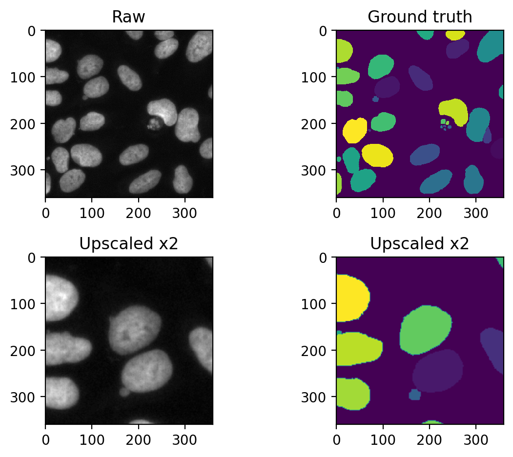
Receptive field#
The receptive field of a convolutional network determines, how large of an area in the input image the deepest layers in the network (highest number of feature maps, lowest number of image size) can see. We can demonstrate this by simply upscaling an input image and check whether stardist is still able to see it:
sample = X_val[0]
sample_upscaled = transform.rescale(sample, 2)[:sample.shape[0], :sample.shape[1]]
sample_upscaled_GT = transform.rescale(Y_val[0], 2)[:sample.shape[0], :sample.shape[1]]
Let’s have a look at the upscaled data:
fig, axes = plt.subplots(ncols=2, nrows=2)
axes[0,0].imshow(sample, cmap='gray')
axes[1,0].imshow(sample_upscaled, cmap='gray')

axes[0,1].imshow(Y_val[0])
axes[1,1].imshow(sample_upscaled_GT)

axes[0,0].set_title('Raw')
axes[1,0].set_title('Upscaled x2')
axes[0,1].set_title('Ground truth')
axes[1,1].set_title('Upscaled x2')
fig.tight_layout()
Exercise 1#
Run the prediction on both images (sample and sample_upscaled) and compare the predictions - what do you observe? Hint: Run the prediction on some data with model.predict_instances()