Basic descriptive statistics

The term descriptive statistics refers to methods that allow summarizing collections of data. To demonstrate the most important methods, we start by defining a dataset first.

measurements = [5, 2, 6, 4, 8, 6, 2, 5, 1, 3, 3, 6]

Measurements of central tendency

We can measure the location of our measurement in space using numpy’s statistics functions and Python’s statistics module.

import numpy as np
import statistics as st
from scipy import stats
import matplotlib.pyplot as plt

average = np.mean(measurements)
average

4.25

median = np.median(measurements)
median

4.5

mode = st.mode(measurements)
mode

6

Measurements of spread

Numpy also allows measuring the spread of measurements.

standard_deviation = np.std(measurements)
standard_deviation

2.0052015692526606

variance = np.var(measurements)
variance

4.020833333333333

np.min(measurements), np.max(measurements)

(1, 8)

np.percentile(measurements, [25, 50, 75])

array([2.75, 4.5 , 6.  ])

np.quantile(measurements, [0.25, .50, .75])

array([2.75, 4.5 , 6.  ])

With the array sorted, it is easier to interpret some of these measurements. We can sort a list like this.

sorted(measurements)

[1, 2, 2, 3, 3, 4, 5, 5, 6, 6, 6, 8]

Skewness

Skewness is a measure of the asymetry of a distribution. Typically, positive values indicate a tail to the right, as shown below, while negative indicate a tail to the left. Values close to zero mean a symetric distribution.

# Fixed seed for reproducibility
np.random.seed(4)

samples = np.random.poisson(lam = average, size = 100)
plt.hist(samples)

(array([20., 21., 17., 13., 12.,  9.,  2.,  2.,  2.,  2.]),
 array([ 1. ,  2.1,  3.2,  4.3,  5.4,  6.5,  7.6,  8.7,  9.8, 10.9, 12. ]),
 <BarContainer object of 10 artists>)

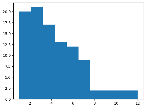
stats.skew(samples)

0.9129973255137396

Let’s check now the skewness of a normal distribution.

samples = np.random.normal(loc = average, scale = standard_deviation, size = 100)
plt.hist(samples)

(array([ 3.,  5., 11., 15., 20., 19., 13.,  6.,  7.,  1.]),
 array([-0.25178483,  0.70243337,  1.65665157,  2.61086978,  3.56508798,
         4.51930618,  5.47352438,  6.42774258,  7.38196079,  8.33617899,
         9.29039719]),
 <BarContainer object of 10 artists>)

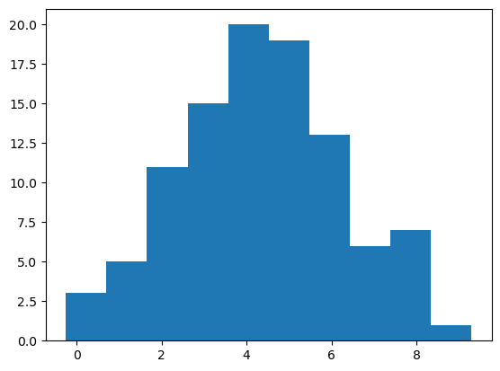
stats.skew(samples)

-0.028758403503365372

Exercise 1

Find out if the median of a sample dataset is always a number within the sample. Use these three examples to elaborate on this:

example1 = [3, 4, 5]

example2 = [3, 4, 4, 5]

example3 = [3, 4, 5, 6]