Subplots with matplotlib
Contents
Subplots with matplotlib#
We already saw that we can use napari to interactively visualize images. Sometimes, we may want to have a static view inside a notebook to consistently share with collaborators or as material in a publication.
Python has many libraries for plotting data, like Matplotlib, Seaborn, plotly and bokeh, to name a few. Some libraries ship plotting function inside them as a convenience. For example, scikit-image and pyclesperanto have a .imshow function, a dedicated plotting function, based on matplotlib, to display intensity and labeled images in notebooks.
In this notebook, we will explain the basics of Matplotlib, probably the most flexible and traditional library to display images and data in Python.
Knowing a bit of its syntax help understanding other higher level libraries.
Importing matplotlib#
For plotting and displaying images, we are usually interested in the pyplot module, so we import it like this:
import matplotlib.pyplot as plt
In this notebook, we will also import a few modules from scikit-image for some basic image processing, and a local colormap derived from the colorcet library.
from skimage import io, filters, measure
Displaying a single image#
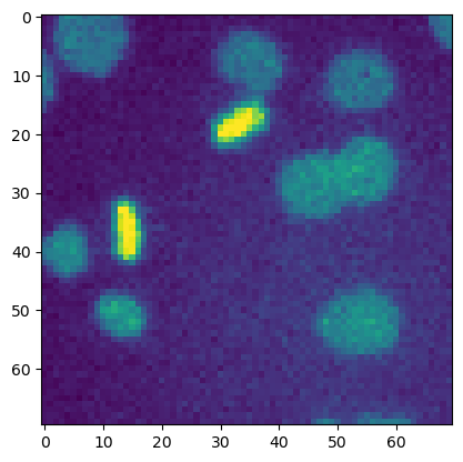
When we want to display a single 2D image, we can just use the function plt.imshow and provide the image as argument.
It implicitly creates a Figure (the cotainer of plot elements) and an Axes (a sub-container of the figure, the plotting area into which most of the objects go).
# Read image from disk
image_cells = io.imread('../../data/mitosis_mod.tif')
plt.imshow(image_cells)
<matplotlib.image.AxesImage at 0x1d7cc9b1640>

We can also explicitly create the Figure and Axes instances beforehand and then add plotting elements, like an image. See other examples of explicitly or implicitly creating figures here.
fig, ax = plt.subplots()
ax.imshow(image_cells)
<matplotlib.image.AxesImage at 0x1d7ccbeedf0>
This difference becomes more relevant when we want to have multiple images/plots in the same figure.
Creating Multiple Subplots#
Let’s read some processed images to display them together afterwards.
image_filtered = io.imread('../../data/mitosis_mod_filtered.tif')
binary_image = io.imread('../../data/mitosis_mod_binary.tif')
label_image = io.imread('../../data/mitosis_mod_labeled.tif')
With the plt.subplots function, we can provide optional arguments (nrwos and ncols) to pre-define a grid of axes.
fig, ax = plt.subplots(nrows = 2, ncols = 2)
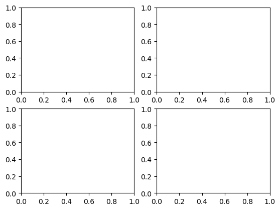
Now, we just have to populate the axes with images or plots, assigning images to the proper axes element by means of row and column indices.
For example, ax[0, 1] points to the first row (row #0) and to the second column (col #1).
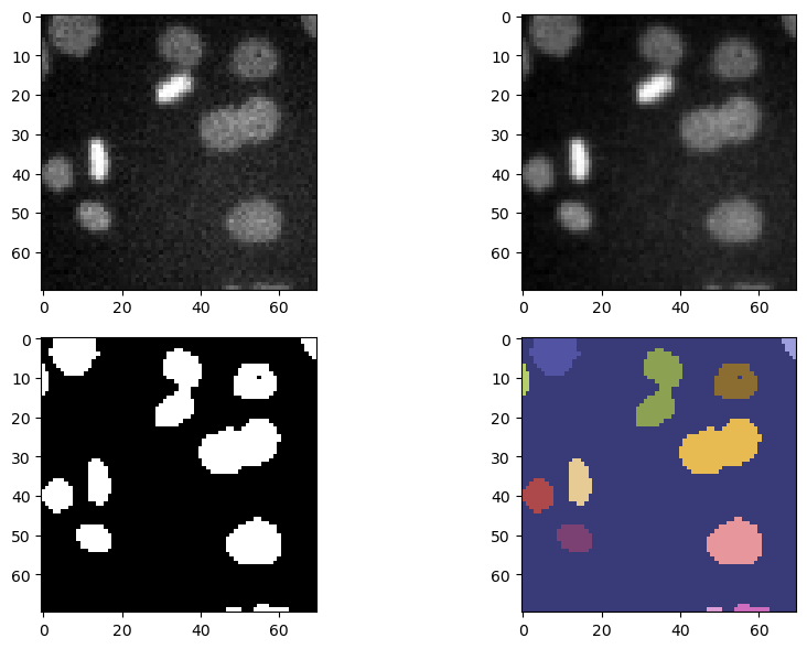
fig, ax = plt.subplots(nrows = 2, ncols = 2, figsize = (10,6))

ax[0, 0].imshow(image_cells, cmap = 'gray')
ax[0, 1].imshow(image_filtered, cmap = 'gray')
ax[1, 0].imshow(binary_image, cmap = 'gray')
ax[1, 1].imshow(label_image, cmap = 'tab20b')

# Handy function to avoid overlap of axes labels
plt.tight_layout()
Other properties of individual axes can be edited like this by providing the right axes indexing to the ax variable.
To get a overview of the available options that can be edited in a figure, take a look at this figure