Segmentation Workflow Example with 3D Data

This notebook applies a custom segmentation workflow to a 3D nuclei image and measure their properties.

from skimage.io import imread
import napari_segment_blobs_and_things_with_membranes as nsbatwm
from napari_skimage_regionprops._regionprops import regionprops_table
import pandas as pd
import napari
viewer = napari.Viewer()

INFO:xmlschema:Resource 'XMLSchema.xsd' is already loaded

Open image and add it to napari

image0_n = imread("../../data/nuclei.tif")
viewer.add_image(image0_n, name="nuclei3d")

<Image layer 'nuclei3d' at 0x1b2dc590e20>

Apply voronoi otsu labeling from ‘nsbatwm’

image1_V = nsbatwm.voronoi_otsu_labeling(image0_n, 9.0, 3.0)
viewer.add_labels(image1_V, name='Result of Voronoi-Otsu-labeling (nsbatwm)')
napari.utils.nbscreenshot(viewer)

Apply remove labels on edges from ‘nsbatwm’

image2_R = nsbatwm.remove_labels_on_edges(image1_V)
viewer.add_labels(
    image2_R, name='Result of Remove labeled objects at the image border (scikit-image, nsbatwm)')
napari.utils.nbscreenshot(viewer)

Measure properties from ‘scikit-image’

To measure some object properties, here we use regionprops_table function from napari_skimage_regionprops, a convenient package based on scikit-image.regionprops that integrates to napari. Another well-suited option for 3D data would be to use SimpleITK by means of the function label_statistics.

The output properties can be displayed in a table format by using the pandas DataFrame class.

df = pd.DataFrame(regionprops_table(image0_n, image2_R, shape = True))
df

	label	area	bbox_area	convex_area	equivalent_diameter	max_intensity	mean_intensity	min_intensity	solidity	extent	feret_diameter_max	local_centroid-0	local_centroid-1	local_centroid-2	standard_deviation_intensity	minor_axis_length	intermediate_axis_length	major_axis_length
0	2	54018	95160	56545	46.900769	55624.0	14464.512237	2656.0	0.955310	0.567654	62.713635	13.364397	25.457755	29.293958	4805.435420	31.327969	52.933836	62.953106
1	5	33789	71400	37316	40.110577	27219.0	11941.699014	3841.0	0.905483	0.473235	57.323643	12.970641	24.381988	25.413922	2634.150462	27.770888	40.471195	58.424627
2	6	37770	84150	40336	41.627736	34332.0	12231.912126	4410.0	0.936384	0.448841	60.942596	14.037225	25.143685	24.855361	2812.426772	30.788439	40.258475	59.120315
3	10	62690	138355	70018	49.287094	46093.0	13604.486840	3177.0	0.895341	0.453110	69.555733	17.141298	29.485404	30.823369	4320.199048	33.433710	53.831092	67.988548
4	12	35227	67840	37057	40.671702	34617.0	12520.697703	5216.0	0.950617	0.519266	56.621551	14.429500	18.455418	25.085531	2672.433396	31.836384	37.536132	57.477872
5	13	50281	96720	53668	45.793281	32910.0	13568.257433	2845.0	0.936890	0.519861	63.039670	14.202084	26.887970	29.218631	3758.117584	30.653051	50.748681	62.747225
6	14	47652	91035	49683	44.980834	47610.0	15270.557668	3367.0	0.959121	0.523447	55.263008	16.303828	24.445417	24.678712	5085.798832	33.553811	50.917972	53.555392
7	15	39960	74307	42190	42.417228	42394.0	12881.410035	3746.0	0.947144	0.537769	53.600373	14.970821	25.792593	23.624575	3322.773305	31.962681	45.374937	53.145880
8	18	41456	78336	43518	42.940087	39406.0	13613.137712	3746.0	0.952617	0.529208	50.813384	15.346850	23.811318	23.456532	3504.742536	33.757661	47.638142	49.489597
9	20	37480	77175	39760	41.520922	36134.0	13623.915715	2656.0	0.942656	0.485649	52.411831	17.442716	22.771798	24.673986	3463.962853	31.691874	45.865526	49.960174
10	21	53894	119662	61516	46.864854	41113.0	14404.345734	3462.0	0.876097	0.450385	68.658576	18.467566	18.107377	32.375292	4509.947285	33.761613	44.762926	71.035177

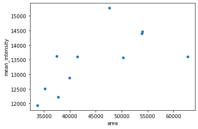
Plot data

Pandas has some built-in plotting capabilities, check more options here.

For a quick demonstration, here we show how to display a scatter plot of two table columns. More customized and stylish plots can be better achieved with dedicated plotting libraries like matplotlib, seaborn, among others.

df.plot.scatter('area', 'mean_intensity')

<AxesSubplot:xlabel='area', ylabel='mean_intensity'>

Save table to disk

Pandas has easy functions to save table to disk. Below, we show how to save a table as a csv file.

df.to_csv('../../data/3D/table_nuclei.csv')

Exercise

Now that you have a complete working workflow, put it inside a function.

Below you find an empty function that should receive an image and return a labeled image. Fill it with the commands used above to have the same output.

def my_segmentation(image):
    """Apply custom 3D nuclei segmentation and return labeled image"""
    
       
    return label_image

Then, run your new function as shown below, passing the input image as argument and adding the output labeled image to napari to check if the result is the same.

image2_R = my_segmentation(image0_n)
viewer.add_labels(image2_R)