(Probabilistic) Noise2Void (2D)

This notebook is a re-implementation of the code for denoising with noise2void as proovided by the authors in this repository. Unlike the original code, this implementation uses pytorch instead of tensorflow. The key idea is to crop small tiles from image data, replace a given pixel with any other pixel in the tile and then try to predict the true intensity of the replaced pixel. Since the intensity of every pixel \(i\) consists of two components noise \(n\) and \(s\) (intensity \(i=n+s\)), the network will inevitably fail to predict the noise component \(n\) of the pixel - thus cleaning up the image in the process.

Source code

Since the torch-implementation of noise2void is currently not (yet) pip-installlable, we simply clone the repository and import the functions provided therein.

!git clone https://github.com/juglab/pn2v.git

fatal: destination path 'pn2v' already exists and is not an empty directory.

import os
os.chdir('pn2v')

import matplotlib.pyplot as plt
import numpy as np
import stackview

from unet.model import UNet
from pn2v import utils
from pn2v import training, prediction
import pn2v.histNoiseModel
from skimage import io
import stackview

device=utils.getDevice()

CUDA available? True

Dataset

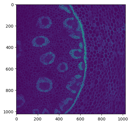
As a training dataset, we’ll use this data of a developing tribolium embryo.

root = '/projects/p038/p_scads_trainings/BIAS/torch_segmentation_denoising_example_data/denoising_example_data'
filename = os.path.join(root, 'convallaria.tif')
data = io.imread(filename)

plt.imshow(data[40])

<matplotlib.image.AxesImage at 0x2b1d4fd87b50>

Training

We next create the model:

# The N2V network requires only a single output unit per pixel
net = UNet(1, depth=3)

Noise2void provides the training.trainNetwork function to run the training. The essential parameters here are the following:

• numOfEpochs: number of epochs to train

• numOfIterations: number of steps in each epochs

• patchSize: size of the patches to extract from the images

• batchSize: number of patches to use in each iteration

model_directory = './model'
os.makedirs(model_directory, exist_ok = True)

# Start training.
trainHist, valHist = training.trainNetwork(net=net, trainData=data, valData=data,
                                           postfix='conv_N2V', directory=model_directory, noiseModel=None,
                                           device=device, numOfEpochs=20, stepsPerEpoch=10, 
                                           virtualBatchSize=20, batchSize=1, learningRate=1e-3)

Epoch 0 finished      
avg. loss: 0.5396011963486671+-(2SEM)0.1632045770490405      
Epoch 1 finished      
avg. loss: 0.14107346385717393+-(2SEM)0.03511942115563338      
Epoch 2 finished      
avg. loss: 0.1530279416590929+-(2SEM)0.03784216142151133      
Epoch 3 finished      
avg. loss: 0.14400796890258788+-(2SEM)0.0405738361070597      
Epoch 4 finished      
avg. loss: 0.12245606444776058+-(2SEM)0.03131022265661264      
Epoch 5 finished      
avg. loss: 0.09631720948964358+-(2SEM)0.02312176777554985      
Epoch 6 finished      
avg. loss: 0.10415804497897625+-(2SEM)0.01675637456608379      
Epoch 7 finished      
avg. loss: 0.12776857577264308+-(2SEM)0.03699295650252412      
Epoch 8 finished      
avg. loss: 0.10771282762289047+-(2SEM)0.03300412868589734      
Epoch 9 finished      
avg. loss: 0.11204689629375934+-(2SEM)0.02957868532185728      
Epoch 10 finished      
avg. loss: 0.0889200784265995+-(2SEM)0.01682425631985288      
Epoch 11 finished      
avg. loss: 0.09613503376021981+-(2SEM)0.01971031434416211      
Epoch 12 finished      
avg. loss: 0.12121303789317608+-(2SEM)0.02920666492861341      
Epoch 13 finished      
avg. loss: 0.12641384545713663+-(2SEM)0.028079695492453025      
Epoch 14 finished      
avg. loss: 0.0830618416890502+-(2SEM)0.015677364268100714      
Epoch 00015: reducing learning rate of group 0 to 5.0000e-04.
Epoch 15 finished      
avg. loss: 0.12371947942301631+-(2SEM)0.03727989255051846      
Epoch 16 finished      
avg. loss: 0.11964833308011294+-(2SEM)0.03351835889931938      
Epoch 17 finished      
avg. loss: 0.12522194683551788+-(2SEM)0.03280974934396423      
Epoch 18 finished      
avg. loss: 0.12407186031341552+-(2SEM)0.040678906442775255      
Epoch 19 finished      
avg. loss: 0.1335150668397546+-(2SEM)0.03227846053322892      
Finished Training      

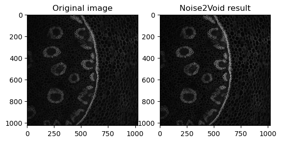
n2vResult = prediction.tiledPredict(data[40], net ,ps=256, overlap=48,
                                        device=device, noiseModel=None)

fig, axes = plt.subplots(ncols=2)

axes[0].imshow(data[40], cmap='gray')
axes[0].set_title('Original image')

axes[1].imshow(n2vResult, cmap='gray')
axes[1].set_title('Noise2Void result')

Text(0.5, 1.0, 'Noise2Void result')

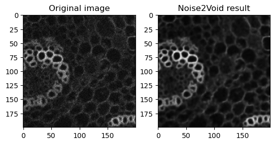
fig, axes = plt.subplots(ncols=2)

axes[0].imshow(data[40][800:1000, 0:200], cmap='gray')
axes[0].set_title('Original image')

axes[1].imshow(n2vResult[800:1000, 0:200], cmap='gray')
axes[1].set_title('Noise2Void result')

Text(0.5, 1.0, 'Noise2Void result')

stackview.curtain(data[40][800:1000, 0:200], n2vResult[800:1000, 0:200], zoom_factor=2)

Process 3D data

Noise2Void generally runs under the assumption, that the noise between neighboring pixels is un-correlated. This assumption is valid in both 3D and 2D. While the performance is probably worse than using a real 3D convolutional network, it is still legitimate too apply noise2void slice by slice to the data stack:

denoised_image = np.zeros_like(data)

for z in range(data.shape[0]):
    denoised_image[z] = prediction.tiledPredict(data[z], net ,ps=256, overlap=48,
                                        device=device, noiseModel=None)

fig, axes = plt.subplots(ncols=2)

axes[0].imshow(data[40, :, :], cmap='gray')
axes[0].set_title('Original image')

axes[1].imshow(denoised_image[40, :, :], cmap='gray')
axes[1].set_title('Noise2Void result')

Text(0.5, 1.0, 'Noise2Void result')

fig, axes = plt.subplots(ncols=2)

axes[0].imshow(data[40, 800:1000, 0:200], cmap='gray')
axes[0].set_title('Original image')

axes[1].imshow(denoised_image[40, 800:1000, 0:200], cmap='gray')
axes[1].set_title('Noise2Void result')

Text(0.5, 1.0, 'Noise2Void result')

stackview.curtain(data[40], denoised_image[40], zoom_factor=0.5)