Going for the GPU

Training of the model in the previous notebook was rather slow, you might have thought. This was the case even if your machine has a GPU available. But don’t be disappointed yet. The truth is that we have not made use of the GPU at all just yet. Usage of devices has to be handled manually by the user in torch. First we will check if torch recognizes any devices it could use for accelerating training.

import torch

cuda_present = torch.cuda.is_available()
ndevices = torch.cuda.device_count()
use_cuda = cuda_present and ndevices > 0
device = torch.device("cuda" if use_cuda else "cpu")  # "cuda:0" ... default device, "cuda:1" would be GPU index 1, "cuda:2" etc
print("number of devices:", ndevices, "\tchosen device:", device, "\tuse_cuda=", use_cuda)

number of devices: 1 	chosen device: cuda 	use_cuda= True

from torch.utils.data import DataLoader
from data import DSBData, get_dsb2018_train_files

from monai.networks.nets import BasicUNet

train_img_files, train_lbl_files = get_dsb2018_train_files()

train_data = DSBData(
    image_files=train_img_files,
    label_files=train_lbl_files,
    target_shape=(256, 256)
)

print(len(train_data))

train_loader = DataLoader(train_data, batch_size=32, shuffle=True, num_workers=1, pin_memory=True)

100%|██████████| 382/382 [00:19<00:00, 19.69it/s]

232

model = BasicUNet(
    spatial_dims=2,
    in_channels=1,
    out_channels=1,
    features=[16, 16, 32, 64, 128, 16],
    act="relu",
    norm="batch",
    dropout=0.25,
)

# Important: transfer the model to the chosen device
model = model.to(device)

BasicUNet features: (16, 16, 32, 64, 128, 16).

Training of a neural network means updating its parameters (weights) using a strategy that involves the gradients of a loss function with respect to the model parameters in order to adjust model weights to minimize this loss.

optimizer = torch.optim.Adam(model.parameters(), lr=1.e-3)
init_params = list(model.parameters())[0].clone().detach()

Such a training is performed by iterating over the batches of the training dataset multiple times. Each full iteration over the dataset is termed an epoch.

max_nepochs = 1
log_interval = 1
model.train(True)

# BCEWithLogitsLoss combines sigmoid + BCELoss for better
# numerical stability. It expects raw unnormalized scores as input which are shaped like 
# B x C x W x D
loss_function = torch.nn.BCEWithLogitsLoss(reduction="mean")

for epoch in range(1, max_nepochs + 1):
    for batch_idx, (X, y) in enumerate(train_loader):
        # the inputs and labels have to be on the same device as the model
        X, y = X.to(device), y.to(device)
        
        optimizer.zero_grad()

        prediction_logits = model(X)
        
        batch_loss = loss_function(prediction_logits, y)

        batch_loss.backward()

        optimizer.step()

        if batch_idx % log_interval == 0:
            print(
                "Train Epoch:",
                epoch,
                "Batch:",
                batch_idx,
                "Total samples processed:",
                (batch_idx + 1) * train_loader.batch_size,
                "Loss:",
                batch_loss.item(),
            )

Train Epoch: 1 Batch: 0 Total samples processed: 32 Loss: 0.7781020402908325
Train Epoch: 1 Batch: 1 Total samples processed: 64 Loss: 0.7558881044387817
Train Epoch: 1 Batch: 2 Total samples processed: 96 Loss: 0.7125054597854614
Train Epoch: 1 Batch: 3 Total samples processed: 128 Loss: 0.673947811126709
Train Epoch: 1 Batch: 4 Total samples processed: 160 Loss: 0.6690397262573242
Train Epoch: 1 Batch: 5 Total samples processed: 192 Loss: 0.6610376834869385
Train Epoch: 1 Batch: 6 Total samples processed: 224 Loss: 0.6330360174179077
Train Epoch: 1 Batch: 7 Total samples processed: 256 Loss: 0.6149089336395264

final_params = list(model.parameters())[0].clone().detach()
assert not torch.allclose(init_params, final_params)

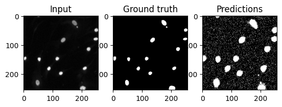
Look at some predictions

Now that the model has been trained for a little bit, we are looking at the predictions again. Usually model training has to be peformed longer, so don’t expect any wonders. Also keep in mind that the predictions here are based on the data the model was trained on. Those predictions might be far better than those on data not used during training. But this is a story for later.

import matplotlib.pyplot as plt

# convert to 0/1 range on each pixel
prediction = torch.nn.functional.sigmoid(prediction_logits)
prediction_binary = (prediction > 0.5).to(torch.uint8)

sidx = 0
plt.subplot(131)
plt.imshow(X[sidx, 0].cpu().numpy(), cmap="gray")
plt.title("Input")

plt.subplot(132)
plt.imshow(y[sidx, 0].cpu().numpy(), cmap="gray")
plt.title("Ground truth")

plt.subplot(133)
plt.imshow(prediction_binary.cpu().detach()[sidx, 0].numpy(), cmap="gray")
plt.title("Predictions")

Text(0.5, 1.0, 'Predictions')

Exercises: Any Differences?

Executing on the CPU versus the GPU should yield no differences other than a speed up in execution times. In the best of all worlds, the GPU version runs training faster at the same quality of prediction. Compare with the last notebook if this is really the case!