Quantiative neighborhood measurements
Contents
Quantiative neighborhood measurements#
In this notebook we demonstrate how to quantify relationships between neighboring cells. We use the neighbor count to remove objects from a label image that are no cells. Afterwards we will measure and visualize the size of cells and the average size of cells in a given neighborhood.
import pyclesperanto_prototype as cle
import numpy as np
from skimage.io import imread
import pandas as pd
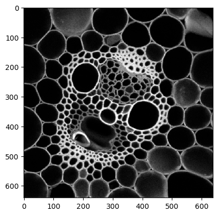
The example image maize_clsm.tif was shared by David Legland and is licensed under CC-BY 4.0 license.
intensity_image = imread('../../data/maize_clsm.tif')
cle.imshow(intensity_image)
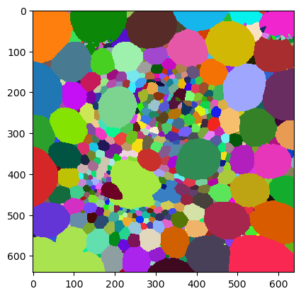
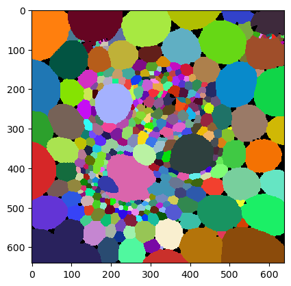
Starting point: Label map#
We use a basic segmentation algorithm to segment the dark objects in the image, hoping these are mostly cells.
binary = cle.binary_not(cle.threshold_otsu(intensity_image))
objects = cle.voronoi_labeling(binary)

cle.imshow(objects, labels=True)
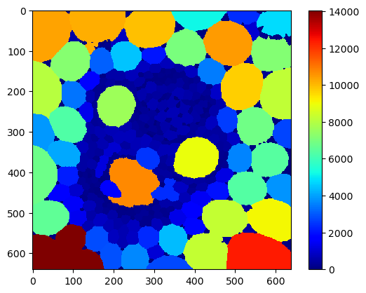
Number of touching neighbor map#
Next, we visualize the number of neighbors in colour.
num_neighbors_map = cle.touching_neighbor_count_map(objects)

cle.imshow(num_neighbors_map,
           colormap='jet',
           colorbar=True)
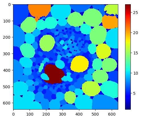
By specifying minimum and maximum display intensity, we can see that most triangular objects, that are presumably no cells, have about 3 neighbors only.
cle.imshow(num_neighbors_map,
           min_display_intensity=0,
           max_display_intensity=6,
           colormap='jet',
           colorbar=True)
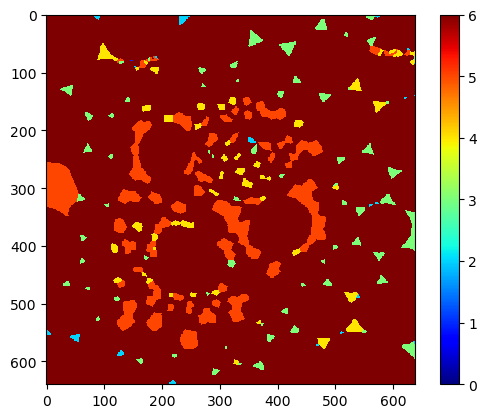
Filtering labels according to measurements#
We can now exclude objects that have < 4 neighbors.
cells = cle.exclude_labels_with_map_values_out_of_range(num_neighbors_map, objects, minimum_value_range=4)

cle.imshow(cells, labels=True)
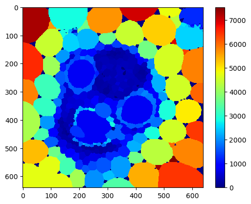
Averaging values over a defined neighborhood#
Now, with a cleaned result, we can measure properties of cells. Note: It would be scientifically questionable to count the number of neighbors now as we used this measurement for filtering the objects.
area_map = cle.pixel_count_map(cells)
cle.imshow(area_map,
           colormap='jet',
           colorbar=True)
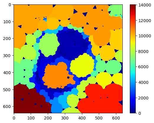
For visualization purposes, we now produce a map that shows the average size and the maximum among neighbors for each cell.
local_mean_area_map = cle.mean_of_touching_neighbors_map(area_map, cells)
cle.imshow(local_mean_area_map,
           colormap='jet',
           colorbar=True)
local_max_area_map = cle.maximum_of_touching_neighbors_map(area_map, cells)
cle.imshow(local_max_area_map,
           colormap='jet',
           colorbar=True)
Tabular neighborhood analysis#
These and similar measurments can also be derived in tabular form.
statistics = cle.statistics_of_labelled_neighbors(cells)

pd.DataFrame(statistics)
| label | touching_neighbor_count | minimum_distance_of_touching_neighbors | average_distance_of_touching_neighbors | maximum_distance_of_touching_neighbors | max_min_distance_ratio_of_touching_neighbors | proximal_neighbor_count_d10 | proximal_neighbor_count_d20 | proximal_neighbor_count_d40 | proximal_neighbor_count_d80 | ... | touching_neighbor_count_dilated_r_10 | minimum_distance_of_touching_neighbors_dilated_r_10 | average_distance_of_touching_neighbors_dilated_r_10 | maximum_distance_of_touching_neighbors_dilated_r_10 | max_min_distance_ratio_of_touching_neighbors_dilated_r_10 | touch_count_sum_dilated_r_10 | minimum_touch_count_dilated_r_10 | maximum_touch_count_dilated_r_10 | minimum_touch_portion_dilated_r_10 | maximum_touch_portion_dilated_r_10 | |
|---|---|---|---|---|---|---|---|---|---|---|---|---|---|---|---|---|---|---|---|---|---|
| 0 | 1 | 4.0 | 60.320210 | 101.840363 | 139.683594 | 2.315701 | 0.0 | 0.0 | 0.0 | 1.0 | ... | 4.0 | 60.131992 | 101.611427 | 138.916809 | 2.310198 | 251.0 | 40.0 | 99.0 | 0.159363 | 0.394422 |
| 1 | 2 | 5.0 | 70.345596 | 102.279503 | 139.683594 | 1.985676 | 0.0 | 0.0 | 0.0 | 1.0 | ... | 5.0 | 69.458466 | 101.834366 | 138.916809 | 1.999998 | 313.0 | 47.0 | 81.0 | 0.150160 | 0.258786 |
| 2 | 3 | 4.0 | 66.247681 | 88.231575 | 105.587234 | 1.593825 | 0.0 | 0.0 | 0.0 | 2.0 | ... | 4.0 | 65.842422 | 88.179047 | 105.653221 | 1.604638 | 231.0 | 54.0 | 67.0 | 0.233766 | 0.290043 |
| 3 | 4 | 5.0 | 62.034245 | 82.326614 | 107.360519 | 1.730665 | 0.0 | 0.0 | 0.0 | 3.0 | ... | 5.0 | 61.471870 | 82.060867 | 107.331879 | 1.746032 | 283.0 | 46.0 | 66.0 | 0.162544 | 0.233216 |
| 4 | 5 | 5.0 | 65.249962 | 80.454788 | 107.360519 | 1.645373 | 0.0 | 0.0 | 0.0 | 3.0 | ... | 5.0 | 65.238731 | 80.336967 | 107.331879 | 1.645217 | 309.0 | 32.0 | 132.0 | 0.103560 | 0.427184 |
| ... | ... | ... | ... | ... | ... | ... | ... | ... | ... | ... | ... | ... | ... | ... | ... | ... | ... | ... | ... | ... | ... |
| 369 | 370 | 4.0 | 6.401806 | 28.644737 | 55.443081 | 8.660537 | 2.0 | 5.0 | 10.0 | 14.0 | ... | 4.0 | 6.355856 | 29.127771 | 55.813652 | 8.781452 | 46.0 | 6.0 | 25.0 | 0.130435 | 0.543478 |
| 370 | 371 | 5.0 | 7.438875 | 17.765903 | 53.682270 | 7.216450 | 4.0 | 4.0 | 9.0 | 14.0 | ... | 5.0 | 7.462044 | 17.792099 | 54.364231 | 7.285434 | 50.0 | 5.0 | 16.0 | 0.100000 | 0.320000 |
| 371 | 372 | 4.0 | 5.430400 | 16.685814 | 47.472179 | 8.741931 | 3.0 | 4.0 | 9.0 | 14.0 | ... | 4.0 | 5.702640 | 17.013132 | 48.531986 | 8.510442 | 26.0 | 5.0 | 8.0 | 0.192308 | 0.307692 |
| 372 | 373 | 2.0 | 8.850188 | 30.322327 | 51.794464 | 5.852357 | 1.0 | 4.0 | 9.0 | 14.0 | ... | 2.0 | 8.285303 | 30.604389 | 52.923477 | 6.387633 | 36.0 | 16.0 | 20.0 | 0.444444 | 0.555556 |
| 373 | 374 | 3.0 | 5.430400 | 22.109964 | 51.449951 | 9.474431 | 2.0 | 4.0 | 9.0 | 14.0 | ... | 3.0 | 5.702640 | 22.457144 | 53.156166 | 9.321326 | 23.0 | 6.0 | 10.0 | 0.260870 | 0.434783 |
374 rows × 64 columns