Quantitative image analysis
Contents
Quantitative image analysis#
After segmenting and labeling objects in an image, we can measure properties of these objects.
See also
Before we can do measurements, we need an image and a corresponding label_image. Therefore, we recapitulate filtering, thresholding and labeling:
import pandas as pd
from skimage.io import imread
from skimage import filters

from skimage import measure
from pyclesperanto_prototype import imshow
# load image
image = imread("../../data/blobs.tif")

# denoising
blurred_image = filters.gaussian(image, sigma=1)

# binarization
threshold = filters.threshold_otsu(blurred_image)
thresholded_image = blurred_image >= threshold

# labeling
label_image = measure.label(thresholded_image)

# visualization
imshow(label_image, labels=True)
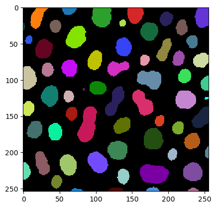
Measurements / region properties#
To read out properties from regions, we use the regionprops function:
# analyse objects
properties = measure.regionprops(label_image, intensity_image=image)
The results are stored as RegionProps objects, which are not very informative:
properties[0:5]
[<skimage.measure._regionprops.RegionProperties at 0x1ecd7842df0>,
 <skimage.measure._regionprops.RegionProperties at 0x1ecd78420a0>,
 <skimage.measure._regionprops.RegionProperties at 0x1ecd7842a90>,
 <skimage.measure._regionprops.RegionProperties at 0x1ecd7842550>,
 <skimage.measure._regionprops.RegionProperties at 0x1ecd78428e0>]
We can reorganize the measurements into a dictionary containing arrays. We introduced them earlier as tables:
statistics = {
    'area':       [p.area               for p in properties],
    'mean':       [p.mean_intensity     for p in properties],
    'major_axis': [p.major_axis_length  for p in properties]
}

statistics
{'area': [429,
  183,
  658,
  433,
  472,
  280,
  75,
  271,
  227,
  27,
  494,
  649,
  96,
  225,
  448,
  397,
  513,
  423,
  268,
  349,
  158,
  406,
  422,
  254,
  503,
  282,
  675,
  176,
  358,
  542,
  599,
  7,
  635,
  192,
  594,
  19,
  264,
  896,
  473,
  239,
  166,
  408,
  413,
  239,
  374,
  647,
  378,
  577,
  66,
  169,
  467,
  612,
  539,
  203,
  556,
  850,
  278,
  213,
  79,
  88,
  52,
  48],
 'mean': [191.44055944055944,
  179.84699453551912,
  205.6048632218845,
  217.5150115473441,
  213.03389830508473,
  205.65714285714284,
  164.16,
  176.0590405904059,
  189.53303964757708,
  149.33333333333334,
  190.0080971659919,
  172.42526964560864,
  166.41666666666666,
  196.8,
  209.03571428571428,
  180.0705289672544,
  194.86939571150097,
  196.27423167848698,
  200.77611940298507,
  190.64756446991404,
  183.69620253164558,
  187.21182266009853,
  202.54028436018956,
  180.5984251968504,
  198.6958250497018,
  189.33333333333334,
  199.07555555555555,
  195.3181818181818,
  197.7877094972067,
  198.760147601476,
  190.85141903171953,
  146.28571428571428,
  193.22204724409448,
  181.83333333333334,
  210.45117845117846,
  150.31578947368422,
  189.93939393939394,
  198.59821428571428,
  205.5137420718816,
  191.59832635983264,
  184.09638554216866,
  179.80392156862746,
  199.94188861985472,
  188.21757322175733,
  195.76470588235293,
  200.70479134466768,
  208.23280423280423,
  201.01213171577123,
  188.36363636363637,
  181.53846153846155,
  167.58886509635974,
  220.0261437908497,
  189.5213358070501,
  199.96059113300493,
  216.93525179856115,
  197.9294117647059,
  190.44604316546761,
  184.52582159624413,
  184.81012658227849,
  182.72727272727272,
  189.53846153846155,
  173.83333333333334],
 'major_axis': [34.77923003414236,
  20.950530036869296,
  30.19848422590625,
  24.508790749585156,
  31.08476574192099,
  20.456703267018653,
  10.455950805204104,
  22.270013595805494,
  18.204772873013326,
  12.678548278670085,
  26.121885258285065,
  33.385906778814366,
  12.546653692400314,
  18.35737770149141,
  26.27274937409412,
  35.8698551687111,
  27.860019629951697,
  28.010713581438814,
  21.468307192278967,
  22.917689441728474,
  15.666167580602863,
  23.865287484124742,
  32.6668803721007,
  19.57228408508096,
  33.24776088170501,
  20.24089328396192,
  36.442424525819675,
  20.498286890054775,
  23.711197998545444,
  29.20849759104235,
  47.75343594118352,
  3.0237157840738176,
  40.67149576429511,
  16.77158509151243,
  28.811758210746788,
  6.09093638927516,
  20.588317981737514,
  54.585718360111564,
  32.95587965343868,
  19.25126182233261,
  16.687880082810175,
  26.756617235381256,
  25.62619404615955,
  18.831258251302966,
  24.783530938010692,
  30.43602504101513,
  23.49797787654461,
  27.804675105924606,
  16.651155953717762,
  17.042194757272345,
  35.316994908476254,
  32.401948630679065,
  30.136816201114012,
  24.67233590691917,
  27.47945909705002,
  41.32954022794983,
  21.637743417307323,
  18.753879494637765,
  18.287488895428375,
  21.673692014391232,
  14.33510391276191,
  16.925659950161798]}
You can also add custom columns by computing your own metric, for example the aspect_ratio:
statistics['aspect_ratio'] = [p.major_axis_length / p.minor_axis_length for p in properties]
Reading those dictionaries of arrays is not very convenient. Thus, we use the pandas library which is a common asset for data scientists.
dataframe = pd.DataFrame(statistics)
dataframe
| area | mean | major_axis | aspect_ratio | |
|---|---|---|---|---|
| 0 | 429 | 191.440559 | 34.779230 | 2.088249 |
| 1 | 183 | 179.846995 | 20.950530 | 1.782168 |
| 2 | 658 | 205.604863 | 30.198484 | 1.067734 |
| 3 | 433 | 217.515012 | 24.508791 | 1.061942 |
| 4 | 472 | 213.033898 | 31.084766 | 1.579415 |
| ... | ... | ... | ... | ... |
| 57 | 213 | 184.525822 | 18.753879 | 1.296143 |
| 58 | 79 | 184.810127 | 18.287489 | 3.173540 |
| 59 | 88 | 182.727273 | 21.673692 | 4.021193 |
| 60 | 52 | 189.538462 | 14.335104 | 2.839825 |
| 61 | 48 | 173.833333 | 16.925660 | 4.417297 |
62 rows × 4 columns
Those dataframes can be saved to disk conveniently:
dataframe.to_csv("blobs_analysis.csv")
Furthermore, one can measure properties from our statistics table using numpy. For example the mean area:
import numpy as np

# measure mean area
np.mean(statistics['area'])
355.3709677419355
Exercises#
Analyse the loaded blobs image.
How many objects are in it?
How large is the largest object?
What are mean and standard deviation of the intensity in the image?
What are mean and standard deviation of the area of the segmented objects?