Exploratory Data Analysis#
Inspiration and some of the parts came from: Python Data Science GitHub repository, MIT License and Introduction to Pandas by Google, Apache 2.0
If running this from Google Colab, uncomment the cell below and run it. Otherwise, just skip it.
#!pip install seaborn
#!pip install watermark
import pandas as pd
import seaborn as sns
from scipy import stats
Learning Objectives:#
descriptive statistics/EDA
corr matrix
For this notebook, we will use the california housing dataframes.
california_housing_dataframe = pd.read_csv("https://download.mlcc.google.com/mledu-datasets/california_housing_train.csv", sep=",")
california_housing_dataframe
| longitude | latitude | housing_median_age | total_rooms | total_bedrooms | population | households | median_income | median_house_value | |
|---|---|---|---|---|---|---|---|---|---|
| 0 | -114.31 | 34.19 | 15.0 | 5612.0 | 1283.0 | 1015.0 | 472.0 | 1.4936 | 66900.0 |
| 1 | -114.47 | 34.40 | 19.0 | 7650.0 | 1901.0 | 1129.0 | 463.0 | 1.8200 | 80100.0 |
| 2 | -114.56 | 33.69 | 17.0 | 720.0 | 174.0 | 333.0 | 117.0 | 1.6509 | 85700.0 |
| 3 | -114.57 | 33.64 | 14.0 | 1501.0 | 337.0 | 515.0 | 226.0 | 3.1917 | 73400.0 |
| 4 | -114.57 | 33.57 | 20.0 | 1454.0 | 326.0 | 624.0 | 262.0 | 1.9250 | 65500.0 |
| ... | ... | ... | ... | ... | ... | ... | ... | ... | ... |
| 16995 | -124.26 | 40.58 | 52.0 | 2217.0 | 394.0 | 907.0 | 369.0 | 2.3571 | 111400.0 |
| 16996 | -124.27 | 40.69 | 36.0 | 2349.0 | 528.0 | 1194.0 | 465.0 | 2.5179 | 79000.0 |
| 16997 | -124.30 | 41.84 | 17.0 | 2677.0 | 531.0 | 1244.0 | 456.0 | 3.0313 | 103600.0 |
| 16998 | -124.30 | 41.80 | 19.0 | 2672.0 | 552.0 | 1298.0 | 478.0 | 1.9797 | 85800.0 |
| 16999 | -124.35 | 40.54 | 52.0 | 1820.0 | 300.0 | 806.0 | 270.0 | 3.0147 | 94600.0 |
17000 rows × 9 columns
Exploring Data#
As shown above, after loading a large DataFrame, it may be a bit hard to have a good overview of what is inside it just by looking at a few rows. Thus, the DataFrame.describe method is useful to show interesting statistics about a DataFrame.
california_housing_dataframe.describe()
| longitude | latitude | housing_median_age | total_rooms | total_bedrooms | population | households | median_income | median_house_value | |
|---|---|---|---|---|---|---|---|---|---|
| count | 17000.000000 | 17000.000000 | 17000.000000 | 17000.000000 | 17000.000000 | 17000.000000 | 17000.000000 | 17000.000000 | 17000.000000 |
| mean | -119.562108 | 35.625225 | 28.589353 | 2643.664412 | 539.410824 | 1429.573941 | 501.221941 | 3.883578 | 207300.912353 |
| std | 2.005166 | 2.137340 | 12.586937 | 2179.947071 | 421.499452 | 1147.852959 | 384.520841 | 1.908157 | 115983.764387 |
| min | -124.350000 | 32.540000 | 1.000000 | 2.000000 | 1.000000 | 3.000000 | 1.000000 | 0.499900 | 14999.000000 |
| 25% | -121.790000 | 33.930000 | 18.000000 | 1462.000000 | 297.000000 | 790.000000 | 282.000000 | 2.566375 | 119400.000000 |
| 50% | -118.490000 | 34.250000 | 29.000000 | 2127.000000 | 434.000000 | 1167.000000 | 409.000000 | 3.544600 | 180400.000000 |
| 75% | -118.000000 | 37.720000 | 37.000000 | 3151.250000 | 648.250000 | 1721.000000 | 605.250000 | 4.767000 | 265000.000000 |
| max | -114.310000 | 41.950000 | 52.000000 | 37937.000000 | 6445.000000 | 35682.000000 | 6082.000000 | 15.000100 | 500001.000000 |
Another useful function is DataFrame.head, which displays the first few records of a DataFrame. You can give it a number of rows to display.
california_housing_dataframe.head(10)
| longitude | latitude | housing_median_age | total_rooms | total_bedrooms | population | households | median_income | median_house_value | |
|---|---|---|---|---|---|---|---|---|---|
| 0 | -114.31 | 34.19 | 15.0 | 5612.0 | 1283.0 | 1015.0 | 472.0 | 1.4936 | 66900.0 |
| 1 | -114.47 | 34.40 | 19.0 | 7650.0 | 1901.0 | 1129.0 | 463.0 | 1.8200 | 80100.0 |
| 2 | -114.56 | 33.69 | 17.0 | 720.0 | 174.0 | 333.0 | 117.0 | 1.6509 | 85700.0 |
| 3 | -114.57 | 33.64 | 14.0 | 1501.0 | 337.0 | 515.0 | 226.0 | 3.1917 | 73400.0 |
| 4 | -114.57 | 33.57 | 20.0 | 1454.0 | 326.0 | 624.0 | 262.0 | 1.9250 | 65500.0 |
| 5 | -114.58 | 33.63 | 29.0 | 1387.0 | 236.0 | 671.0 | 239.0 | 3.3438 | 74000.0 |
| 6 | -114.58 | 33.61 | 25.0 | 2907.0 | 680.0 | 1841.0 | 633.0 | 2.6768 | 82400.0 |
| 7 | -114.59 | 34.83 | 41.0 | 812.0 | 168.0 | 375.0 | 158.0 | 1.7083 | 48500.0 |
| 8 | -114.59 | 33.61 | 34.0 | 4789.0 | 1175.0 | 3134.0 | 1056.0 | 2.1782 | 58400.0 |
| 9 | -114.60 | 34.83 | 46.0 | 1497.0 | 309.0 | 787.0 | 271.0 | 2.1908 | 48100.0 |
Or DataFrame.tail, which displays the last few records of a DataFrame:
california_housing_dataframe.tail()
| longitude | latitude | housing_median_age | total_rooms | total_bedrooms | population | households | median_income | median_house_value | |
|---|---|---|---|---|---|---|---|---|---|
| 16995 | -124.26 | 40.58 | 52.0 | 2217.0 | 394.0 | 907.0 | 369.0 | 2.3571 | 111400.0 |
| 16996 | -124.27 | 40.69 | 36.0 | 2349.0 | 528.0 | 1194.0 | 465.0 | 2.5179 | 79000.0 |
| 16997 | -124.30 | 41.84 | 17.0 | 2677.0 | 531.0 | 1244.0 | 456.0 | 3.0313 | 103600.0 |
| 16998 | -124.30 | 41.80 | 19.0 | 2672.0 | 552.0 | 1298.0 | 478.0 | 1.9797 | 85800.0 |
| 16999 | -124.35 | 40.54 | 52.0 | 1820.0 | 300.0 | 806.0 | 270.0 | 3.0147 | 94600.0 |
Correletaion Matrix#
Consider the table of measurements below.
blobs_statistics = pd.read_csv('../../data/blobs_statistics.csv', index_col=0)
blobs_statistics.head()
| area | mean_intensity | minor_axis_length | major_axis_length | eccentricity | extent | feret_diameter_max | equivalent_diameter_area | bbox-0 | bbox-1 | bbox-2 | bbox-3 | |
|---|---|---|---|---|---|---|---|---|---|---|---|---|
| 0 | 422 | 192.379147 | 16.488550 | 34.566789 | 0.878900 | 0.586111 | 35.227830 | 23.179885 | 0 | 11 | 30 | 35 |
| 1 | 182 | 180.131868 | 11.736074 | 20.802697 | 0.825665 | 0.787879 | 21.377558 | 15.222667 | 0 | 53 | 11 | 74 |
| 2 | 661 | 205.216339 | 28.409502 | 30.208433 | 0.339934 | 0.874339 | 32.756679 | 29.010538 | 0 | 95 | 28 | 122 |
| 3 | 437 | 216.585812 | 23.143996 | 24.606130 | 0.339576 | 0.826087 | 26.925824 | 23.588253 | 0 | 144 | 23 | 167 |
| 4 | 476 | 212.302521 | 19.852882 | 31.075106 | 0.769317 | 0.863884 | 31.384710 | 24.618327 | 0 | 237 | 29 | 256 |
After measuring many features / properties, it is often common that some of them are strongly correlated and may not bring much new information. In pandas, we can calculate correlation among columns like this.
blobs_statistics.corr()
| area | mean_intensity | minor_axis_length | major_axis_length | eccentricity | extent | feret_diameter_max | equivalent_diameter_area | bbox-0 | bbox-1 | bbox-2 | bbox-3 | |
|---|---|---|---|---|---|---|---|---|---|---|---|---|
| area | 1.000000 | 0.548612 | 0.890649 | 0.895282 | -0.192147 | -0.267454 | 0.916652 | 0.975964 | -0.066508 | -0.081937 | 0.034083 | -0.003961 |
| mean_intensity | 0.548612 | 1.000000 | 0.657131 | 0.440678 | -0.362592 | -0.011555 | 0.487183 | 0.611103 | 0.015188 | 0.217484 | 0.069184 | 0.266504 |
| minor_axis_length | 0.890649 | 0.657131 | 1.000000 | 0.664507 | -0.566486 | -0.037872 | 0.716706 | 0.937795 | -0.163017 | -0.056785 | -0.077817 | 0.015790 |
| major_axis_length | 0.895282 | 0.440678 | 0.664507 | 1.000000 | 0.168454 | -0.551362 | 0.995196 | 0.880909 | -0.010743 | -0.128821 | 0.093556 | -0.057776 |
| eccentricity | -0.192147 | -0.362592 | -0.566486 | 0.168454 | 1.000000 | -0.432629 | 0.103529 | -0.272402 | 0.257938 | -0.060467 | 0.253671 | -0.076793 |
| extent | -0.267454 | -0.011555 | -0.037872 | -0.551362 | -0.432629 | 1.000000 | -0.517428 | -0.278453 | -0.076688 | 0.048511 | -0.128149 | 0.019310 |
| feret_diameter_max | 0.916652 | 0.487183 | 0.716706 | 0.995196 | 0.103529 | -0.517428 | 1.000000 | 0.911211 | -0.025173 | -0.122607 | 0.080054 | -0.049283 |
| equivalent_diameter_area | 0.975964 | 0.611103 | 0.937795 | 0.880909 | -0.272402 | -0.278453 | 0.911211 | 1.000000 | -0.107059 | -0.096706 | -0.004660 | -0.018489 |
| bbox-0 | -0.066508 | 0.015188 | -0.163017 | -0.010743 | 0.257938 | -0.076688 | -0.025173 | -0.107059 | 1.000000 | 0.050957 | 0.993418 | 0.053563 |
| bbox-1 | -0.081937 | 0.217484 | -0.056785 | -0.128821 | -0.060467 | 0.048511 | -0.122607 | -0.096706 | 0.050957 | 1.000000 | 0.032728 | 0.996062 |
| bbox-2 | 0.034083 | 0.069184 | -0.077817 | 0.093556 | 0.253671 | -0.128149 | 0.080054 | -0.004660 | 0.993418 | 0.032728 | 1.000000 | 0.041855 |
| bbox-3 | -0.003961 | 0.266504 | 0.015790 | -0.057776 | -0.076793 | 0.019310 | -0.049283 | -0.018489 | 0.053563 | 0.996062 | 0.041855 | 1.000000 |
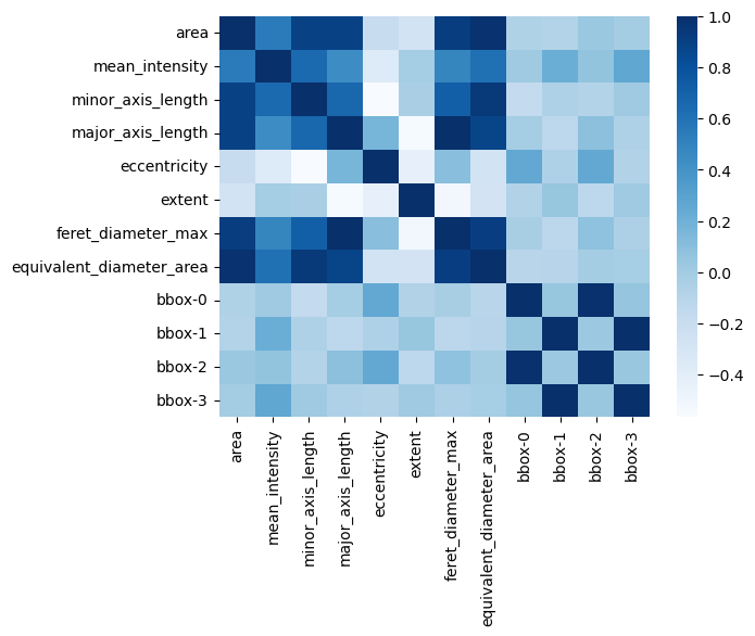
It can be hard to read in numeric format. I wonder if there is beter way how to look at the data?
Below we take a quick shortcut to seaborn to show how the correlation can be displayed as a heatmap.
# calculate the correlation matrix on the numeric columns
corr = blobs_statistics.select_dtypes('number').corr()

# plot the heatmap
sns.heatmap(corr, cmap="Blues", annot=False)
<Axes: >
Watermark
from watermark import watermark
watermark(iversions=True, globals_=globals())
print(watermark())
print(watermark(packages="watermark,numpy,pandas,seaborn,pivottablejs"))
Last updated: 2023-08-24T14:26:10.347260+02:00

Python implementation: CPython
Python version       : 3.9.17
IPython version      : 8.14.0

Compiler    : MSC v.1929 64 bit (AMD64)
OS          : Windows
Release     : 10
Machine     : AMD64
Processor   : Intel64 Family 6 Model 165 Stepping 2, GenuineIntel
CPU cores   : 16
Architecture: 64bit

watermark   : 2.4.3
numpy       : 1.23.5
pandas      : 2.0.3
seaborn     : 0.12.2
pivottablejs: 0.9.0