Images in python

This notebook was based on 00_images_are_arrays from the Scipy-2023-image-nalaysis repository under BSD 3-Clause “New” or “Revised” License.

In this notebook we will show how to open images and how to display them. In order to do that, we need to introduce three python libraries: scikit-image, numpy and matplotlib.

Breifly, scikit-image is a collection of python functions for image processing, numpy is the fundamental package for scientific computing with python and matplotlib is the standard library for plotting with python.

Images are numpy arrays

Images are represented in scikit-image using standard numpy arrays. This allows maximum inter-operability with other libraries in the scientific Python ecosystem, such as matplotlib and scipy.

Below we import numpy and give it an alias: ‘np’.

import numpy as np

We can build a 1D numpy array with np.array()

numpy_array = np.array(
    [0, 1, 2, 3]
)
numpy_array

array([0, 1, 2, 3])

To build a 2D numpy array, we simply add another level of square brackets:

numpy_array = np.array(
    [
        [1, 2, 3],
        [4, 5, 6]
    ]
)
numpy_array

array([[1, 2, 3],
       [4, 5, 6]])

We can check the shape of this arrays with .shape. This returns a tuple with the number os rows and the number of columns of our numpy array.

numpy_array.shape

(2, 3)

A 2D numpy array can alrady be understood as an image, where the values correspond to intensity of each pixel. Let’s use .imshow() matplotlib to visualize it as an image. The cmap='gray' argument defines that the values should be displayed with a grayscale palette.

import matplotlib.pyplot as plt
plt.imshow(numpy_array, cmap='gray')

<matplotlib.image.AxesImage at 0x185b6a974f0>

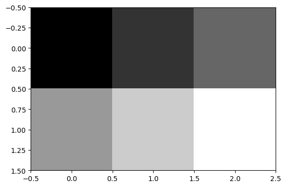
See? Images are numpy arrays!

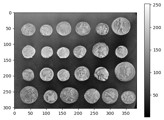
The same holds for “real-world” images. Take a look at some example images loaded from scikit-image below.

from skimage import data

coins = data.coins()

plt.imshow(coins, cmap='gray')
plt.colorbar()

<matplotlib.colorbar.Colorbar at 0x185b7e82a90>

We can check that coins is an array by assessing type.

type(coins)

numpy.ndarray

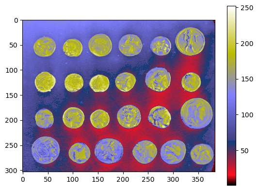
We can display the same image with different “look-up tables” or “colormaps”. These images are not true color images, they just translate different intensity values to specified colors from a colorbar instead of a grayscale bar. The pixel values remain the same.

Sometimes viewing the same image under different perspectives may be insightful. For example, it may be more obvious to spot the background heterogeneity by looking at the image below than the one displayed in grayscale above.

plt.imshow(coins, cmap='gist_stern')
plt.colorbar()

<matplotlib.colorbar.Colorbar at 0x185b7ef9850>

N-dimensional images

Some images have more than 2 dimensions. For example, a true color image is a 3D array, where the last dimension has size 3 (or 4) and represents the red, green, and blue channels.

A z-stack is also a 3D array, where one of the dimensions correspond to z-slices.

Furhtermore, microscopy images may have multiple channels acquired from different detectors and these are also typically stored as an extra dimension.

Let’s check an example below.

cells_3D = data.cells3d()
cells_3D.shape

(60, 2, 256, 256)

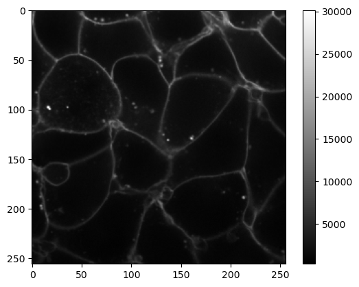
This iamge has 4 dimensions. We can display a z-slice and a channel by providing indices to the array. For example, let’s load the 30th slice and the first channel.

Notice that, in Python, indexing starts from 0, so the first channel has index 0 and the 30th slice has index 29!

cells_membranes_slice = cells_3D[29, 0]

plt.imshow(cells_membranes_slice, cmap='gray')
plt.colorbar()

<matplotlib.colorbar.Colorbar at 0x185bccce7f0>

Exercise

Get a z-slice from the other channel and display it with a the colormap 'magma'.