Object Size, Shape & Intensity#
This notebook shows you (1) how to determine the size of either a single object or all of the objects in an instance segmentation dataset, (2) how to index the dictionaries that are the output of skimage.regionprops and (3) shows some of the ‘underbelly’ workings of regionprops by first showing you how to implement scipy.ndimage.labeled_comprehension and then showing you how to write an intensity standard deviation function yourself.
from __future__ import division, print_function

import numpy as np
from skimage.io import imread, imshow
from skimage.measure import regionprops
from scipy.ndimage import labeled_comprehension
import matplotlib.pyplot as plt

%matplotlib inline
Load Data#
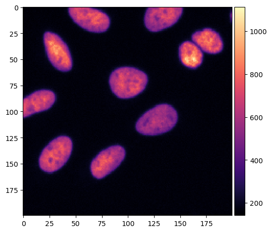
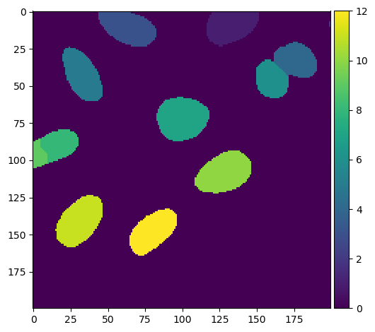
We will use an instance segmentation that is the result of a voronoi otsu labeling method applied to a small crop of the skimage.data.cells3d().
input_image = imread('data/cropped_raw_image.tif')
imshow(input_image, cmap='magma')
/Users/ryan/mambaforge/envs/devbio-napari-env/lib/python3.9/site-packages/skimage/io/_plugins/matplotlib_plugin.py:150: UserWarning: Low image data range; displaying image with stretched contrast.
  lo, hi, cmap = _get_display_range(image)
<matplotlib.image.AxesImage at 0x19b58ac10>
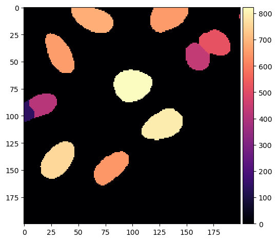
voronoi_otsu_segmentation = imread('data/instance_segmentation.tif')
imshow(voronoi_otsu_segmentation)
<matplotlib.image.AxesImage at 0x19b721730>
Extract Features#
Apply regionprops from skimage.measure to the labeled image. This will return a list of dictionaries. Each dictionary corresponds to a single object (i.e., nucleus) in the labeled image. Below I show you how to index each dictionary with a key to retrieve a specific feature (i.e., eccentricity) that is measured by regionprops.
regprops = regionprops(voronoi_otsu_segmentation)
for i in range(len(regprops)):
    print(regprops[i].eccentricity)
0.7903767216752334
1.0
0.8591188380687891
0.6774692528388002
0.8682019435379323
0.637161426772526
0.5656238837964573
0.6409503067624858
0.8470599794547478
0.780930799306185
0.8003925438834633
0.8451613028758732
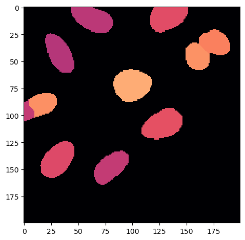
Colorcode your image by feature measurements#
In the following cell, I show you how to create an image where the colormap values correspond to a chosen feature value using python indexing tricks.
This can be very useful for creating visuals for presentations to be shown in parallel with plots or other quantification visuals.
eccentricity_image = np.copy(voronoi_otsu_segmentation).astype(float)
for i in range(len(regprops)):
    eccentricity_image[eccentricity_image == i+1] = regprops[i].axis_minor_length / regprops[i].axis_major_length
You can save the image you just created either as a ‘.tif’ file using skimage.io.imsave or simply by displaying it as an image plot using skimage.io.imshow followed by plt.savefig. If you use the second approach, be sure to define an appropriate resolution (i.e., dpi) for presentations/figures.
imshow(eccentricity_image, cmap = 'magma')
plt.tight_layout()
plt.savefig('eccentricity_image.png', dpi = 300)
Mean Intensity#
We will use the segmentation result to calculate the mean intensity of one object in the orginal image. We will look at the object with the segmention label ID \(8\). To do this, we will use a neat indexing trick.
mean_intenstity = np.mean(input_image[voronoi_otsu_segmentation == 8])
mean_intenstity
614.1990291262136
Minimum & Maximum Intensities#
This time assign the index that we used for the mean intensity to a variable so that we can use it to calculate the object’s minimum and maximum intensities in the same fashion.
mask = input_image[voronoi_otsu_segmentation == 8]
minimum_intensity = np.min(mask)
minimum_intensity
386
maximum_intensity = np.max(mask)
maximum_intensity
821
In the following cell, retrieve the minimum and maximum intensity of each of the labeled objects from regprops using the correct keys for the dictionaries (if you do not know them, either check the function’s docstring by clicking ‘shift tab’ inside the round parentheses or go to the skimage.measure API (https://scikit-image.org/docs/dev/api/skimage.measure.html#skimage.measure.regionprops).
Labeled Comprehension#
We can use a function from the scipy.ndimage library called labeled_comprehension if you wish to only run one function that measures a feature, here np.mean to retrieve the mean pixel intensity, for all objects in an instance segmentation. labeled_comprehension requires many inputs so read the docstring and carefully think about the correct data to pass.
labels = np.unique(voronoi_otsu_segmentation) # this function finds all of the values present in an array
labels
array([ 0, 1, 2, 3, 4, 5, 6, 7, 8, 9, 10, 11, 12], dtype=uint8)
labels = labels[labels > 0] # index out background value(s)
labels
array([ 1, 2, 3, 4, 5, 6, 7, 8, 9, 10, 11, 12], dtype=uint8)
mean_intensities = labeled_comprehension(input_image,
                                         voronoi_otsu_segmentation,
                                         labels,
                                         np.mean,
                                         int,
                                         0)
Object Size#
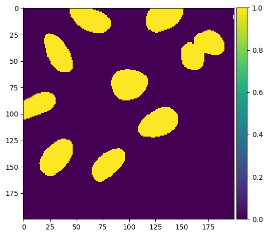
Here we want calculate the size, in pixels, of each object in an instance segmentation. To do this using labeled_comprehension we need to use a boolean image instead of the input image.
Once we have areas in terms of pixel counts, we can then convert them to \(\mu\)m\(^2\) if we know the \(x\) and \(y\) resolutions from the microscope (I have chosen the resolution randomly).
boolean_image = voronoi_otsu_segmentation.astype(bool)
imshow(boolean_image.astype(int))
<matplotlib.image.AxesImage at 0x19b8a8fd0>
In the next cell, we again use labeled_comprehension to apply a single function to each labeled object. Subsequent cells show how you can rescale from pixel areas (i.e., counts) to \(\mu\)m\(^2\) area measurements.
pixel_areas = labeled_comprehension(boolean_image,
                                    voronoi_otsu_segmentation,
                                    labels,
                                    np.sum,
                                    int,
                                    0)
pixel_areas
array([652, 4, 684, 521, 655, 440, 824, 412, 141, 792, 758, 645])
x_resolution = 0.2
y_resolution = 0.2

unit_pixel = x_resolution * y_resolution
unit_pixel
0.04000000000000001
square_micrometer_area = pixel_areas * unit_pixel
square_micrometer_area
array([26.08,  0.16, 27.36, 20.84, 26.2 , 17.6 , 32.96, 16.48,  5.64,
       31.68, 30.32, 25.8 ])
We can again create an image where the colormap reflects the measured feature (\(\mu\)m\(^2\) area).
area_image = np.copy(voronoi_otsu_segmentation).astype(float)
for i in labels:
    area_image[area_image == i] = pixel_areas[i-1]
imshow(area_image, cmap = 'magma')
/Users/ryan/mambaforge/envs/devbio-napari-env/lib/python3.9/site-packages/skimage/io/_plugins/matplotlib_plugin.py:150: UserWarning: Float image out of standard range; displaying image with stretched contrast.
  lo, hi, cmap = _get_display_range(image)
<matplotlib.image.AxesImage at 0x19b997400>
Plotting Your Features#
Before diving into statistical analysis, sometimes it is good to plot the values of your features as a histogram or scatter plot as a sanity check to ensure that you did not somehow impart bias into your analysis.
Below we will plot two of the features we extracted as histograms and then as a scatter plot comparing them. These plots are very simple, but if you would like to customize the axes, colors, etc. look at the following documentation:
https://matplotlib.org/stable/api/_as_gen/matplotlib.pyplot.hist.html
https://matplotlib.org/stable/api/_as_gen/matplotlib.pyplot.scatter.html
plt.hist(mean_intensities)
plt.show()
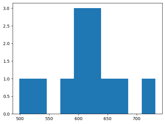
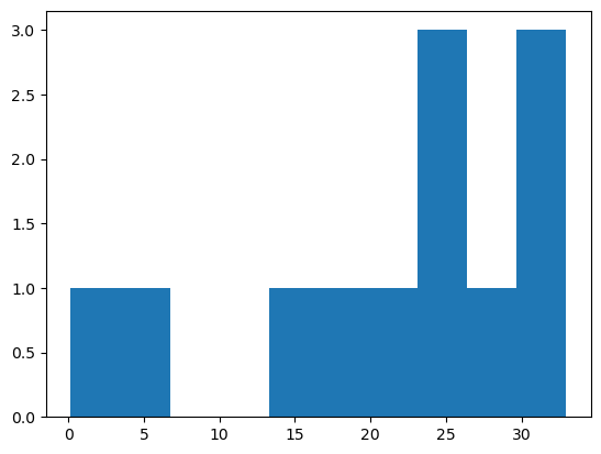
plt.hist(square_micrometer_area)
plt.show()
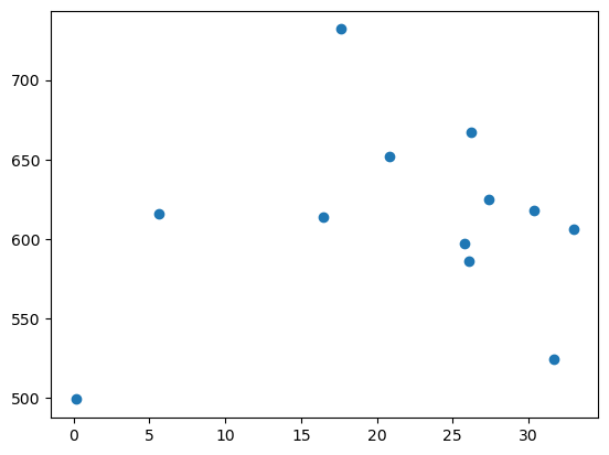
plt.scatter(square_micrometer_area, mean_intensities)
plt.show()
Exercise#
To better understand the ‘inner workings’ of regionprops and/or labeled_comprehension works’, write a function using a for loop, np.unique and np.std to retrieve the standard deviation of intensity values for each object in the image used above. Then apply your function, plot a histogram of its results and compare it to the results of from regionprops and/or labeled_comprehension.
def object_standard_deviation(input_image, segmented_image):

    from numpy import unique, zeros_like, std

    labels = unique(segmented_image)
    labels = labels[labels > 0]

    stds = zeros_like(labels, dtype=float)

    counter = 0
    for i in labels:
        i_mask = input_image[segmented_image == i]
        i_std = std(i_mask)
        stds[counter] = i_std
        counter += 1

    return stds
stds = object_standard_deviation(input_image, voronoi_otsu_segmentation)
stds
array([ 84.36602844,  21.45198126,  95.63218092, 132.03439707,
       139.25476677, 153.20006971,  81.87191519,  87.66097093,
        86.30787008,  53.90184463,  91.3030485 ,  98.35668465])
lc_stds = labeled_comprehension(input_image, voronoi_otsu_segmentation, labels, np.std, out_dtype=float, default=0)
lc_stds
array([ 84.36602844,  21.45198126,  95.63218092, 132.03439707,
       139.25476677, 153.20006971,  81.87191519,  87.66097093,
        86.30787008,  53.90184463,  91.3030485 ,  98.35668465])