Cropping images

When working with microscopy images, it often makes limited sense to process the whole image. We typically crop out interesting regions and process them in detail. In this context, it is important to understand that often times, images in Python are actually simply numpy arrays - which means we can use the same indexing and slicing operations as we have seen for lists and tuples.

from skimage.io import imread, imshow
import numpy as np

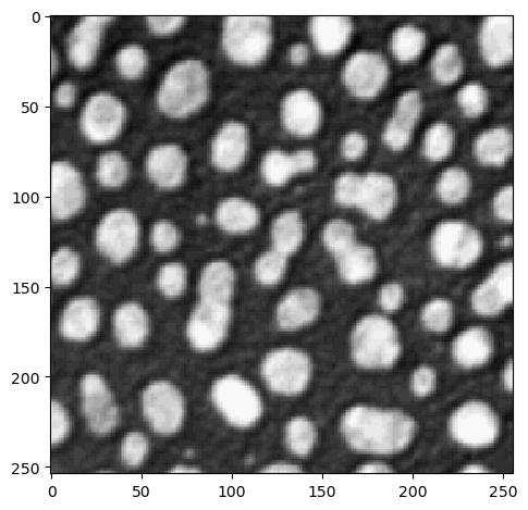
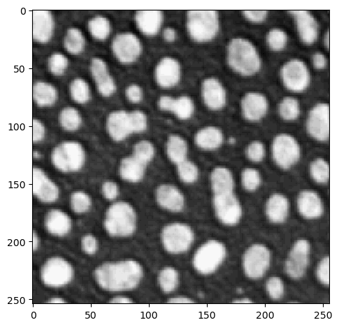
image = imread("../../data/blobs.tif")

Numpy arrays - and thus, images loaded as numpy arrays - have some attributes assigned to them. For instance, ay numpy array has the following attributes we can inspect:

• array.shape: the shape of the array, i.e. the number of elements in each dimension

• array.size: the total number of elements in the array

• array.dtype: the data type of the array ( like int, float, bool, etc.)

For images, before we can crop an image, we may want to know its precise shape (dimensions):

image.shape

(254, 256)

You can visualize images in Jupyter notebooks using the imshow function from scikit-image:

imshow(image)

<matplotlib.image.AxesImage at 0x1fb7748adf0>

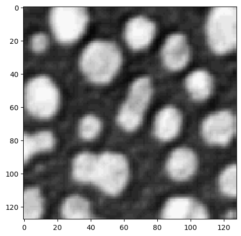
Cropping images works exactly like cropping lists and tuples:

cropped_image1 = image[0:128]

imshow(cropped_image1)

<matplotlib.image.AxesImage at 0x1fb7750b4c0>

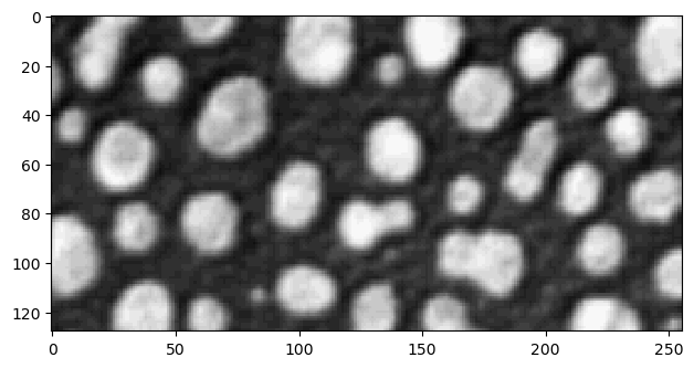
To crop the image in the second dimension as well, we add a , in the square brackets:

cropped_image2 = image[0:128, 128:]

imshow(cropped_image2)

<matplotlib.image.AxesImage at 0x1fb7757eee0>

Sub-sampling images

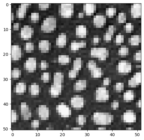
Also step sizes can be specified as if we would process lists and tuples. Technically, we are sub-sampling the image in this case. We sample a subset of the original pixels:

sampled_image = image[::5, ::5]

imshow(sampled_image)

<matplotlib.image.AxesImage at 0x1fb77604520>

Flipping images

Negative step sizes flip the image.

flipped_image = image[::, ::-1]

imshow(flipped_image)

<matplotlib.image.AxesImage at 0x1fb777fa370>

Numpy operations

You can apply element-wise mathematical operations in images:

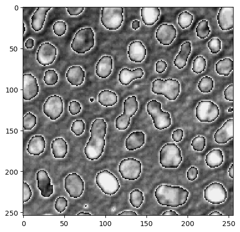
multiplied_image = image * 2
imshow(multiplied_image)

<matplotlib.image.AxesImage at 0x1fb776e4670>

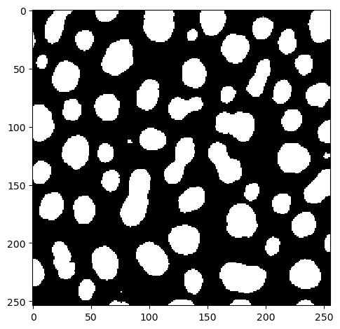
thresholded_image = image > 128
imshow(thresholded_image)

<matplotlib.image.AxesImage at 0x1fb7775ab20>

Exercise 1

Open the banana020.tif data set and crop out the region where the banana slice is located.

Exercise 2

Look at the multiplied_image from above. Why does the image look this way? Hint: Have a look at image.max() (the maximum intensity in the array), multiplied_image.max() as well as image.dtype (the data type of the array).