Parametric maps
Contents
Parametric maps#
For data visualization, parametric maps or feature images, can be useful. This notebook demonstrates how parametric maps can be made. In such parametric images, pixel intensity corresponds to measurements of the objects, for example area.
import numpy as np
import pyclesperanto_prototype as cle
from skimage.io import imread
from skimage.measure import regionprops, regionprops_table
from skimage.util import map_array
from napari_segment_blobs_and_things_with_membranes import voronoi_otsu_labeling
Starting point for drawing parametric maps is always a label image.
image = imread("../../data/BBBC007_batch/17P1_POS0013_D_1UL.tif")
labels = voronoi_otsu_labeling(image)
labels

|
nsbatwm made image
|
Parametric maps using scikit-image#
You can now compute your own measurement for each object and then visualize it in a parametric map image, for example using scikit-image’s regionprops() for computing the measurements.
statistics_table = regionprops_table(cle.pull(labels), properties=('label', 'area',))
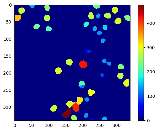
Area map#
area_map = map_array(
        cle.pull(labels),
        statistics_table['label'],
        statistics_table['area'],
        )

cle.imshow(area_map, colorbar=True, color_map="jet")
C:\Users\rober\miniconda3\envs\devbio-napari-env4\lib\site-packages\pyclesperanto_prototype\_tier9\_imshow.py:46: UserWarning: The imshow parameter color_map is deprecated. Use colormap instead.
  warnings.warn("The imshow parameter color_map is deprecated. Use colormap instead.")

Parametric maps in pyclesperanto#
Simpler access, also to more advanced methods for generating parametric maps are available in pyclesperanto. It comes with some maps built-in. For example the pixel count map which is identical to the above shown area map in case the pixel size is 1.
pixel_count_map = cle.pixel_count_map(labels)

cle.imshow(pixel_count_map, color_map='jet', colorbar=True)
C:\Users\rober\miniconda3\envs\devbio-napari-env4\lib\site-packages\pyclesperanto_prototype\_tier9\_imshow.py:46: UserWarning: The imshow parameter color_map is deprecated. Use colormap instead.
  warnings.warn("The imshow parameter color_map is deprecated. Use colormap instead.")
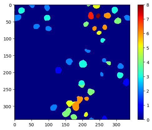
Advanced methods for studying cells in tissues allow for counting for example the number of neighboring cells in a given radius.
neighbor_count_map = cle.proximal_neighbor_count_map(labels, max_distance=50)

cle.imshow(neighbor_count_map, color_map='jet', colorbar=True)
Visualization in napari#
To visualize the parametric images on top of the original image, using napari is recommended.
import napari

viewer = napari.Viewer()

viewer.add_image(image)
area_map_layer = viewer.add_image(area_map, opacity=0.2, blending="additive", colormap="turbo")

napari.utils.nbscreenshot(viewer)

area_map_layer.opacity = 0.9

napari.utils.nbscreenshot(viewer)

Exercise#
Modify the code above to measure the major_axis_length of the objects and visualize the measurements in color in napari. The documentation of regionprops might be useful:
regionprops?
Signature:
regionprops(
    label_image,
    intensity_image=None,
    cache=True,
    coordinates=None,
    *,
    extra_properties=None,
)
Docstring:
Measure properties of labeled image regions.

Parameters
----------
label_image : (M, N[, P]) ndarray
    Labeled input image. Labels with value 0 are ignored.

    .. versionchanged:: 0.14.1
        Previously, ``label_image`` was processed by ``numpy.squeeze`` and
        so any number of singleton dimensions was allowed. This resulted in
        inconsistent handling of images with singleton dimensions. To
        recover the old behaviour, use
        ``regionprops(np.squeeze(label_image), ...)``.
intensity_image : (M, N[, P][, C]) ndarray, optional
    Intensity (i.e., input) image with same size as labeled image, plus
    optionally an extra dimension for multichannel data. Currently,
    this extra channel dimension, if present, must be the last axis.
    Default is None.

    .. versionchanged:: 0.18.0
        The ability to provide an extra dimension for channels was added.
cache : bool, optional
    Determine whether to cache calculated properties. The computation is
    much faster for cached properties, whereas the memory consumption
    increases.
coordinates : DEPRECATED
    This argument is deprecated and will be removed in a future version
    of scikit-image.

    See :ref:`Coordinate conventions <numpy-images-coordinate-conventions>`
    for more details.

    .. deprecated:: 0.16.0
        Use "rc" coordinates everywhere. It may be sufficient to call
        ``numpy.transpose`` on your label image to get the same values as
        0.15 and earlier. However, for some properties, the transformation
        will be less trivial. For example, the new orientation is
        :math:`\frac{\pi}{2}` plus the old orientation.
extra_properties : Iterable of callables
    Add extra property computation functions that are not included with
    skimage. The name of the property is derived from the function name,
    the dtype is inferred by calling the function on a small sample.
    If the name of an extra property clashes with the name of an existing
    property the extra property wil not be visible and a UserWarning is
    issued. A property computation function must take a region mask as its
    first argument. If the property requires an intensity image, it must
    accept the intensity image as the second argument.

Returns
-------
properties : list of RegionProperties
    Each item describes one labeled region, and can be accessed using the
    attributes listed below.

Notes
-----
The following properties can be accessed as attributes or keys:

**area** : int
    Number of pixels of the region.
**area_bbox** : int
    Number of pixels of bounding box.
**area_convex** : int
    Number of pixels of convex hull image, which is the smallest convex
    polygon that encloses the region.
**area_filled** : int
    Number of pixels of the region will all the holes filled in. Describes
    the area of the image_filled.
**axis_major_length** : float
    The length of the major axis of the ellipse that has the same
    normalized second central moments as the region.
**axis_minor_length** : float
    The length of the minor axis of the ellipse that has the same
    normalized second central moments as the region.
**bbox** : tuple
    Bounding box ``(min_row, min_col, max_row, max_col)``.
    Pixels belonging to the bounding box are in the half-open interval
    ``[min_row; max_row)`` and ``[min_col; max_col)``.
**centroid** : array
    Centroid coordinate tuple ``(row, col)``.
**centroid_local** : array
    Centroid coordinate tuple ``(row, col)``, relative to region bounding
    box.
**centroid_weighted** : array
    Centroid coordinate tuple ``(row, col)`` weighted with intensity
    image.
**centroid_weighted_local** : array
    Centroid coordinate tuple ``(row, col)``, relative to region bounding
    box, weighted with intensity image.
**coords** : (N, 2) ndarray
    Coordinate list ``(row, col)`` of the region.
**eccentricity** : float
    Eccentricity of the ellipse that has the same second-moments as the
    region. The eccentricity is the ratio of the focal distance
    (distance between focal points) over the major axis length.
    The value is in the interval [0, 1).
    When it is 0, the ellipse becomes a circle.
**equivalent_diameter_area** : float
    The diameter of a circle with the same area as the region.
**euler_number** : int
    Euler characteristic of the set of non-zero pixels.
    Computed as number of connected components subtracted by number of
    holes (input.ndim connectivity). In 3D, number of connected
    components plus number of holes subtracted by number of tunnels.
**extent** : float
    Ratio of pixels in the region to pixels in the total bounding box.
    Computed as ``area / (rows * cols)``
**feret_diameter_max** : float
    Maximum Feret's diameter computed as the longest distance between
    points around a region's convex hull contour as determined by
    ``find_contours``. [5]_
**image** : (H, J) ndarray
    Sliced binary region image which has the same size as bounding box.
**image_convex** : (H, J) ndarray
    Binary convex hull image which has the same size as bounding box.
**image_filled** : (H, J) ndarray
    Binary region image with filled holes which has the same size as
    bounding box.
**image_intensity** : ndarray
    Image inside region bounding box.
**inertia_tensor** : ndarray
    Inertia tensor of the region for the rotation around its mass.
**inertia_tensor_eigvals** : tuple
    The eigenvalues of the inertia tensor in decreasing order.
**intensity_max** : float
    Value with the greatest intensity in the region.
**intensity_mean** : float
    Value with the mean intensity in the region.
**intensity_min** : float
    Value with the least intensity in the region.
**label** : int
    The label in the labeled input image.
**moments** : (3, 3) ndarray
    Spatial moments up to 3rd order::

        m_ij = sum{ array(row, col) * row^i * col^j }

    where the sum is over the `row`, `col` coordinates of the region.
**moments_central** : (3, 3) ndarray
    Central moments (translation invariant) up to 3rd order::

        mu_ij = sum{ array(row, col) * (row - row_c)^i * (col - col_c)^j }

    where the sum is over the `row`, `col` coordinates of the region,
    and `row_c` and `col_c` are the coordinates of the region's centroid.
**moments_hu** : tuple
    Hu moments (translation, scale and rotation invariant).
**moments_normalized** : (3, 3) ndarray
    Normalized moments (translation and scale invariant) up to 3rd order::

        nu_ij = mu_ij / m_00^[(i+j)/2 + 1]

    where `m_00` is the zeroth spatial moment.
**moments_weighted** : (3, 3) ndarray
    Spatial moments of intensity image up to 3rd order::

        wm_ij = sum{ array(row, col) * row^i * col^j }

    where the sum is over the `row`, `col` coordinates of the region.
**moments_weighted_central** : (3, 3) ndarray
    Central moments (translation invariant) of intensity image up to
    3rd order::

        wmu_ij = sum{ array(row, col) * (row - row_c)^i * (col - col_c)^j }

    where the sum is over the `row`, `col` coordinates of the region,
    and `row_c` and `col_c` are the coordinates of the region's weighted
    centroid.
**moments_weighted_hu** : tuple
    Hu moments (translation, scale and rotation invariant) of intensity
    image.
**moments_weighted_normalized** : (3, 3) ndarray
    Normalized moments (translation and scale invariant) of intensity
    image up to 3rd order::

        wnu_ij = wmu_ij / wm_00^[(i+j)/2 + 1]

    where ``wm_00`` is the zeroth spatial moment (intensity-weighted area).
**orientation** : float
    Angle between the 0th axis (rows) and the major
    axis of the ellipse that has the same second moments as the region,
    ranging from `-pi/2` to `pi/2` counter-clockwise.
**perimeter** : float
    Perimeter of object which approximates the contour as a line
    through the centers of border pixels using a 4-connectivity.
**perimeter_crofton** : float
    Perimeter of object approximated by the Crofton formula in 4
    directions.
**slice** : tuple of slices
    A slice to extract the object from the source image.
**solidity** : float
    Ratio of pixels in the region to pixels of the convex hull image.

Each region also supports iteration, so that you can do::

  for prop in region:
      print(prop, region[prop])

See Also
--------
label

References
----------
.. [1] Wilhelm Burger, Mark Burge. Principles of Digital Image Processing:
       Core Algorithms. Springer-Verlag, London, 2009.
.. [2] B. Jähne. Digital Image Processing. Springer-Verlag,
       Berlin-Heidelberg, 6. edition, 2005.
.. [3] T. H. Reiss. Recognizing Planar Objects Using Invariant Image
       Features, from Lecture notes in computer science, p. 676. Springer,
       Berlin, 1993.
.. [4] https://en.wikipedia.org/wiki/Image_moment
.. [5] W. Pabst, E. Gregorová. Characterization of particles and particle
       systems, pp. 27-28. ICT Prague, 2007.
       https://old.vscht.cz/sil/keramika/Characterization_of_particles/CPPS%20_English%20version_.pdf

Examples
--------
>>> from skimage import data, util
>>> from skimage.measure import label, regionprops
>>> img = util.img_as_ubyte(data.coins()) > 110
>>> label_img = label(img, connectivity=img.ndim)
>>> props = regionprops(label_img)
>>> # centroid of first labeled object
>>> props[0].centroid
(22.72987986048314, 81.91228523446583)
>>> # centroid of first labeled object
>>> props[0]['centroid']
(22.72987986048314, 81.91228523446583)

Add custom measurements by passing functions as ``extra_properties``

>>> from skimage import data, util
>>> from skimage.measure import label, regionprops
>>> import numpy as np
>>> img = util.img_as_ubyte(data.coins()) > 110
>>> label_img = label(img, connectivity=img.ndim)
>>> def pixelcount(regionmask):
...     return np.sum(regionmask)
>>> props = regionprops(label_img, extra_properties=(pixelcount,))
>>> props[0].pixelcount
7741
>>> props[1]['pixelcount']
42
File:      c:\users\rober\miniconda3\envs\devbio-napari-env4\lib\site-packages\skimage\measure\_regionprops.py
Type:      function