Quantitative image analysis using scikit-image
Contents
Quantitative image analysis using scikit-image#
After segmenting and labeling objects in an image, we can measure properties of these objects.
See also
Before we can do measurements, we need an image and a corresponding label_image. Therefore, we recapitulate filtering, thresholding and labeling:
from skimage.io import imread
from skimage import filters

from skimage import measure
from pyclesperanto_prototype import imshow
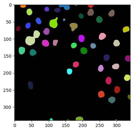
As an example image we will use an extracgt from the BBBC007 dataset image set version 1 (Jones et al., Proc. ICCV Workshop on Computer Vision for Biomedical Image Applications, 2005), available from the Broad Bioimage Benchmark Collection [Ljosa et al., Nature Methods, 2012].
# load image
image = imread("../../data/BBBC007_batch/20P1_POS0010_D_1UL.tif")

# denoising
blurred_image = filters.gaussian(image, sigma=3)

# binarization
threshold = filters.threshold_otsu(blurred_image)
thresholded_image = blurred_image >= threshold

# labeling
label_image = measure.label(thresholded_image)

# visualization
imshow(label_image, labels=True)
Measurements / region properties#
To read out properties from regions, we use the regionprops_table function. To see which features can be measured, please refer to the documentation of regionprops.
# analyse objects
properties = measure.regionprops_table(label_image, intensity_image=image,
                                      properties=('area', 'intensity_mean', 'major_axis_length', 'minor_axis_length'))
properties
{'area': array([139, 360,  43, 140, 144, 194, 251, 310, 276, 160, 283, 539, 237,
         51, 211, 402, 156, 278, 273, 972, 320, 305, 326, 207, 294, 224,
        213, 327, 319, 291, 263, 238, 250, 277, 264, 226, 267, 300, 290,
        282, 307,  84, 315, 206,  45,  33,  16]),
 'intensity_mean': array([ 96.54676259,  86.61388889,  91.48837209,  73.74285714,
         89.375     ,  85.72680412, 100.03984064, 106.14516129,
        113.82246377,  98.30625   , 110.24381625,  93.82931354,
         96.18987342,  64.23529412,  94.84834123, 101.45273632,
         81.39102564, 115.72661871, 108.32967033,  98.72016461,
        120.04375   , 104.26885246, 114.30674847,  81.94202899,
        114.47619048,  88.33482143,  95.05633803,  93.26911315,
        105.5830721 , 110.10309278, 102.33079848, 105.47478992,
        100.256     , 118.20938628,  88.06060606,  93.76548673,
        107.54681648, 104.21333333,  92.9137931 , 104.87943262,
        101.10423453,  86.86904762,  91.13333333,  94.26213592,
         68.37777778,  76.72727273,  76.75      ]),
 'major_axis_length': array([17.50410401, 35.74680768, 12.96788442, 18.94050837, 13.63930773,
        17.90434696, 19.59960381, 21.68348763, 21.49587402, 15.04257295,
        19.82178058, 30.75560175, 20.41073678,  8.50599893, 18.74314548,
        24.25603866, 16.09112371, 21.44453279, 19.89817937, 57.31103495,
        22.67697926, 21.09018439, 22.07441256, 19.11287595, 19.7177777 ,
        18.16615339, 17.24876979, 22.54114086, 21.04530156, 19.60688318,
        19.3948345 , 18.37158206, 18.95328718, 21.73074014, 20.92467079,
        18.07876584, 19.0661401 , 21.47445636, 24.74551721, 20.70344031,
        20.15554708, 14.82486664, 20.92709533, 23.38187856,  9.40637134,
        10.72427534,  7.74596669]),
 'minor_axis_length': array([10.2927697 , 14.98312426,  4.35157341, 10.31440443, 13.45853236,
        13.82984942, 16.30411403, 18.35228668, 16.38949971, 13.54106251,
        18.25604373, 23.86964025, 14.83203512,  7.60835863, 14.35375932,
        22.37062728, 12.36945499, 16.66114148, 17.48026603, 25.5023541 ,
        18.03965907, 18.41775182, 18.80848118, 14.11734515, 19.05302222,
        15.69558924, 15.74682632, 18.5781835 , 19.31001227, 18.97935324,
        17.28272373, 16.96009368, 16.78921681, 16.2409953 , 16.12063476,
        15.98698808, 17.88121627, 17.8176564 , 14.9985119 , 17.41327927,
        19.45870689,  7.62239333, 19.20928278, 11.66966783,  6.27644472,
         4.17456784,  2.78388218])}
You can also add custom measurements by computing your own metric, for example the aspect_ratio:
properties['aspect_ratio'] = properties["major_axis_length"] / properties["minor_axis_length"]

properties['aspect_ratio']
array([1.70062136, 2.38580466, 2.98004496, 1.83631624, 1.01343203,
       1.29461619, 1.20212627, 1.18151422, 1.31156377, 1.11088572,
       1.0857654 , 1.288482  , 1.37612517, 1.11798081, 1.30580046,
       1.08428067, 1.30087572, 1.28709865, 1.13832246, 2.2472841 ,
       1.25706252, 1.14510091, 1.17364142, 1.35385767, 1.03488977,
       1.157405  , 1.09538071, 1.21331242, 1.08986474, 1.03306382,
       1.12220937, 1.08322409, 1.12889645, 1.33801776, 1.29800539,
       1.13084252, 1.0662664 , 1.20523462, 1.64986482, 1.18894552,
       1.03581123, 1.94490969, 1.08942617, 2.0036456 , 1.49867827,
       2.56895462, 2.78243337])
Reading those dictionaries of arrays is not very convenient. Thus, we use the pandas library which is a common asset for data scientists.
import pandas as pd

dataframe = pd.DataFrame(properties)
dataframe
| area | intensity_mean | major_axis_length | minor_axis_length | aspect_ratio | |
|---|---|---|---|---|---|
| 0 | 139 | 96.546763 | 17.504104 | 10.292770 | 1.700621 |
| 1 | 360 | 86.613889 | 35.746808 | 14.983124 | 2.385805 |
| 2 | 43 | 91.488372 | 12.967884 | 4.351573 | 2.980045 |
| 3 | 140 | 73.742857 | 18.940508 | 10.314404 | 1.836316 |
| 4 | 144 | 89.375000 | 13.639308 | 13.458532 | 1.013432 |
| 5 | 194 | 85.726804 | 17.904347 | 13.829849 | 1.294616 |
| 6 | 251 | 100.039841 | 19.599604 | 16.304114 | 1.202126 |
| 7 | 310 | 106.145161 | 21.683488 | 18.352287 | 1.181514 |
| 8 | 276 | 113.822464 | 21.495874 | 16.389500 | 1.311564 |
| 9 | 160 | 98.306250 | 15.042573 | 13.541063 | 1.110886 |
| 10 | 283 | 110.243816 | 19.821781 | 18.256044 | 1.085765 |
| 11 | 539 | 93.829314 | 30.755602 | 23.869640 | 1.288482 |
| 12 | 237 | 96.189873 | 20.410737 | 14.832035 | 1.376125 |
| 13 | 51 | 64.235294 | 8.505999 | 7.608359 | 1.117981 |
| 14 | 211 | 94.848341 | 18.743145 | 14.353759 | 1.305800 |
| 15 | 402 | 101.452736 | 24.256039 | 22.370627 | 1.084281 |
| 16 | 156 | 81.391026 | 16.091124 | 12.369455 | 1.300876 |
| 17 | 278 | 115.726619 | 21.444533 | 16.661141 | 1.287099 |
| 18 | 273 | 108.329670 | 19.898179 | 17.480266 | 1.138322 |
| 19 | 972 | 98.720165 | 57.311035 | 25.502354 | 2.247284 |
| 20 | 320 | 120.043750 | 22.676979 | 18.039659 | 1.257063 |
| 21 | 305 | 104.268852 | 21.090184 | 18.417752 | 1.145101 |
| 22 | 326 | 114.306748 | 22.074413 | 18.808481 | 1.173641 |
| 23 | 207 | 81.942029 | 19.112876 | 14.117345 | 1.353858 |
| 24 | 294 | 114.476190 | 19.717778 | 19.053022 | 1.034890 |
| 25 | 224 | 88.334821 | 18.166153 | 15.695589 | 1.157405 |
| 26 | 213 | 95.056338 | 17.248770 | 15.746826 | 1.095381 |
| 27 | 327 | 93.269113 | 22.541141 | 18.578184 | 1.213312 |
| 28 | 319 | 105.583072 | 21.045302 | 19.310012 | 1.089865 |
| 29 | 291 | 110.103093 | 19.606883 | 18.979353 | 1.033064 |
| 30 | 263 | 102.330798 | 19.394835 | 17.282724 | 1.122209 |
| 31 | 238 | 105.474790 | 18.371582 | 16.960094 | 1.083224 |
| 32 | 250 | 100.256000 | 18.953287 | 16.789217 | 1.128896 |
| 33 | 277 | 118.209386 | 21.730740 | 16.240995 | 1.338018 |
| 34 | 264 | 88.060606 | 20.924671 | 16.120635 | 1.298005 |
| 35 | 226 | 93.765487 | 18.078766 | 15.986988 | 1.130843 |
| 36 | 267 | 107.546816 | 19.066140 | 17.881216 | 1.066266 |
| 37 | 300 | 104.213333 | 21.474456 | 17.817656 | 1.205235 |
| 38 | 290 | 92.913793 | 24.745517 | 14.998512 | 1.649865 |
| 39 | 282 | 104.879433 | 20.703440 | 17.413279 | 1.188946 |
| 40 | 307 | 101.104235 | 20.155547 | 19.458707 | 1.035811 |
| 41 | 84 | 86.869048 | 14.824867 | 7.622393 | 1.944910 |
| 42 | 315 | 91.133333 | 20.927095 | 19.209283 | 1.089426 |
| 43 | 206 | 94.262136 | 23.381879 | 11.669668 | 2.003646 |
| 44 | 45 | 68.377778 | 9.406371 | 6.276445 | 1.498678 |
| 45 | 33 | 76.727273 | 10.724275 | 4.174568 | 2.568955 |
| 46 | 16 | 76.750000 | 7.745967 | 2.783882 | 2.782433 |
Those dataframes can be saved to disk conveniently:
dataframe.to_csv("../../data/BBBC007_analysis.csv")
Furthermore, one can measure properties from our statistics table using numpy. For example the mean area:
import numpy as np

# measure mean area
np.mean(properties['area'])
253.36170212765958
Exercises#
Analyse the loaded blobs image.
How many objects are in it?
How large is the largest object?
What are mean and standard deviation of the image?
What are mean and standard deviation of the area of the segmented objects?