Segmentation Workflow Example with 3D Data
Contents
Segmentation Workflow Example with 3D Data#
This notebook applies a custom segmentation workflow to a 3D nuclei image and measure their properties.
from skimage.io import imread
import napari_segment_blobs_and_things_with_membranes as nsbatwm
from napari_skimage_regionprops._regionprops import regionprops_table
import pandas as pd
import napari
viewer = napari.Viewer()
WARNING: DirectWrite: CreateFontFaceFromHDC() failed (Indicates an error in an input file such as a font file.) for QFontDef(Family="8514oem", pointsize=12, pixelsize=20, styleHint=5, weight=50, stretch=100, hintingPreference=0) LOGFONT("8514oem", lfWidth=0, lfHeight=-20) dpi=240
C:\Miniconda\envs\devbio-napari-env\lib\site-packages\napari_tools_menu\__init__.py:168: FutureWarning: Public access to Window.qt_viewer is deprecated and will be removed in
v0.5.0. It is considered an "implementation detail" of the napari
application, not part of the napari viewer model. If your use case
requires access to qt_viewer, please open an issue to discuss.
  self.tools_menu = ToolsMenu(self, self.qt_viewer.viewer)
Open image and add it to napari#
image0_n = imread("../../data/3D/nuclei.tif")
viewer.add_image(image0_n, name="nuclei3d")
<Image layer 'nuclei3d' at 0x153f7b1a340>
Apply voronoi otsu labeling from ‘nsbatwm’#
image1_V = nsbatwm.voronoi_otsu_labeling(image0_n, 9.0, 3.0)
viewer.add_labels(image1_V, name='Result of Voronoi-Otsu-labeling (nsbatwm)')
napari.utils.nbscreenshot(viewer)

Apply remove labels on edges from ‘nsbatwm’#
image2_R = nsbatwm.remove_labels_on_edges(image1_V)
viewer.add_labels(
    image2_R, name='Result of Remove labeled objects at the image border (scikit-image, nsbatwm)')
napari.utils.nbscreenshot(viewer)

Measure properties from ‘scikit-image’#
To measure some object properties, here we use regionprops_table function from napari_skimage_regionprops, a convenient package based on scikit-image.regionprops that integrates to napari. Another well-suited option for 3D data would be to use SimpleITK by means of the function label_statistics.
The output properties can be displayed in a table format by using the pandas DataFrame class.
df = pd.DataFrame(regionprops_table(image0_n, image2_R, shape = True))
df
| label | area | bbox_area | convex_area | equivalent_diameter | max_intensity | mean_intensity | min_intensity | solidity | extent | feret_diameter_max | local_centroid-0 | local_centroid-1 | local_centroid-2 | standard_deviation_intensity | minor_axis_length | intermediate_axis_length | major_axis_length | |
|---|---|---|---|---|---|---|---|---|---|---|---|---|---|---|---|---|---|---|
| 0 | 2 | 54018 | 95160 | 56545 | 46.900769 | 55624.0 | 14464.512237 | 2656.0 | 0.955310 | 0.567654 | 62.713635 | 13.364397 | 25.457755 | 29.293958 | 4805.435420 | 31.327969 | 52.933836 | 62.953106 |
| 1 | 5 | 33789 | 71400 | 37316 | 40.110577 | 27219.0 | 11941.699014 | 3841.0 | 0.905483 | 0.473235 | 57.323643 | 12.970641 | 24.381988 | 25.413922 | 2634.150462 | 27.770888 | 40.471195 | 58.424627 |
| 2 | 6 | 37770 | 84150 | 40336 | 41.627736 | 34332.0 | 12231.912126 | 4410.0 | 0.936384 | 0.448841 | 60.942596 | 14.037225 | 25.143685 | 24.855361 | 2812.426772 | 30.788439 | 40.258475 | 59.120315 |
| 3 | 10 | 62690 | 138355 | 70018 | 49.287094 | 46093.0 | 13604.486840 | 3177.0 | 0.895341 | 0.453110 | 69.555733 | 17.141298 | 29.485404 | 30.823369 | 4320.199048 | 33.433710 | 53.831092 | 67.988548 |
| 4 | 12 | 35227 | 67840 | 37057 | 40.671702 | 34617.0 | 12520.697703 | 5216.0 | 0.950617 | 0.519266 | 56.621551 | 14.429500 | 18.455418 | 25.085531 | 2672.433396 | 31.836384 | 37.536132 | 57.477872 |
| 5 | 13 | 50281 | 96720 | 53668 | 45.793281 | 32910.0 | 13568.257433 | 2845.0 | 0.936890 | 0.519861 | 63.039670 | 14.202084 | 26.887970 | 29.218631 | 3758.117584 | 30.653051 | 50.748681 | 62.747225 |
| 6 | 14 | 47652 | 91035 | 49683 | 44.980834 | 47610.0 | 15270.557668 | 3367.0 | 0.959121 | 0.523447 | 55.263008 | 16.303828 | 24.445417 | 24.678712 | 5085.798832 | 33.553811 | 50.917972 | 53.555392 |
| 7 | 15 | 39960 | 74307 | 42190 | 42.417228 | 42394.0 | 12881.410035 | 3746.0 | 0.947144 | 0.537769 | 53.600373 | 14.970821 | 25.792593 | 23.624575 | 3322.773305 | 31.962681 | 45.374937 | 53.145880 |
| 8 | 18 | 41456 | 78336 | 43518 | 42.940087 | 39406.0 | 13613.137712 | 3746.0 | 0.952617 | 0.529208 | 50.813384 | 15.346850 | 23.811318 | 23.456532 | 3504.742536 | 33.757661 | 47.638142 | 49.489597 |
| 9 | 20 | 37480 | 77175 | 39760 | 41.520922 | 36134.0 | 13623.915715 | 2656.0 | 0.942656 | 0.485649 | 52.411831 | 17.442716 | 22.771798 | 24.673986 | 3463.962853 | 31.691874 | 45.865526 | 49.960174 |
| 10 | 21 | 53894 | 119662 | 61516 | 46.864854 | 41113.0 | 14404.345734 | 3462.0 | 0.876097 | 0.450385 | 68.658576 | 18.467566 | 18.107377 | 32.375292 | 4509.947285 | 33.761613 | 44.762926 | 71.035177 |
Plot data#
Pandas has some built-in plotting capabilities, check more options here.
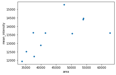
For a quick demonstration, here we show how to display a scatter plot of two table columns. More customized and stylish plots can be better achieved with dedicated plotting libraries like matplotlib, seaborn, among others.
df.plot.scatter('area', 'mean_intensity')
<AxesSubplot:xlabel='area', ylabel='mean_intensity'>
Save table to disk#
Pandas has easy functions to save table to disk. Below, we show how to save a table as a csv file.
df.to_csv('../../data/3D/table_nuclei.csv')
Exercise#
Now that you have a complete working workflow, put it inside a function.
Below you find an empty function that should receive an image and return a labeled image. Fill it with the commands used above to have the same output.
def my_segmentation(image):
    """Apply custom 3D nuclei segmentation and return labeled image"""


    return label_image
Then, run your new function as shown below, passing the input image as argument and adding the output labeled image to napari to check if the result is the same.
image2_R = my_segmentation(image0_n)
viewer.add_labels(image2_R)
Finally save the labeled image to disk with the name ‘nuclei_labels’. Check the function below to find out how to do it.
from skimage.io import imsave

imsave?
Signature: imsave(fname, arr, plugin=None, check_contrast=True, **plugin_args)
Docstring:
Save an image to file.

Parameters
----------
fname : str or pathlib.Path
    Target filename.
arr : ndarray of shape (M,N) or (M,N,3) or (M,N,4)
    Image data.
plugin : str, optional
    Name of plugin to use.  By default, the different plugins are
    tried (starting with imageio) until a suitable
    candidate is found.  If not given and fname is a tiff file, the
    tifffile plugin will be used.
check_contrast : bool, optional
    Check for low contrast and print warning (default: True).

Other Parameters
----------------
plugin_args : keywords
    Passed to the given plugin.

Notes
-----
When saving a JPEG, the compression ratio may be controlled using the
``quality`` keyword argument which is an integer with values in [1, 100]
where 1 is worst quality and smallest file size, and 100 is best quality
and largest file size (default 75).  This is only available when using
the PIL and imageio plugins.
File:      c:\miniconda\envs\devbio-napari-env\lib\site-packages\skimage\io\_io.py
Type:      function