Interactive unsupervised object classification in Napari

In this exercise we will perfom interactive feature plotting and manual selection, Dimensionality Reduction with UMAP and Clustering with HDBSCAN to assign objects (nuclei) to different classes in napari. We will use the napari plugin napari-clusters-plotter plugin.

Getting started

Open a terminal window and activate your conda environment:

mamba activate napari25

Afterwards, start up Napari:

napari

Load the “BBBC007 v1” example dataset from the menu File > Open Sample > napari clusters plotter > BBBC007 v1 dataset.

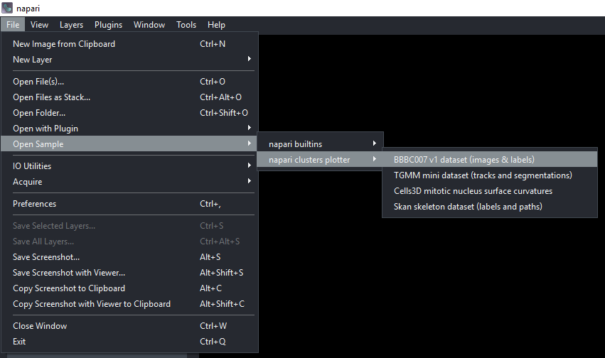
This dataset contains several images of nuclei and segmentation results with features already extracted and stored in each Labels layer. The dataset is from the Broad Bioimage Benchmark Collection.

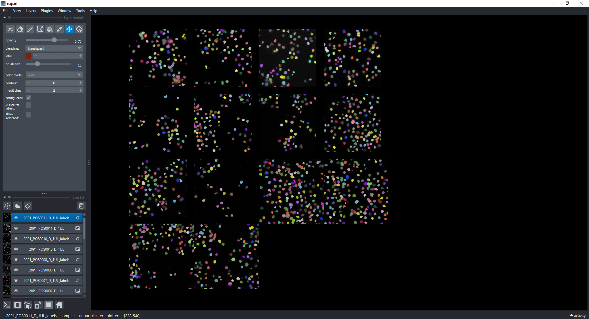
You should see the following layers in the napari canvas:

Plotting Features in napari

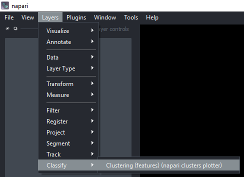
Open the napari-clusters-plotter Plotter via Layers > Visualize > Plot & select features (napari clusters plotter).

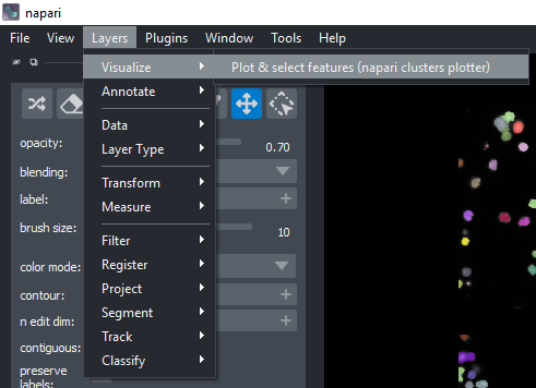
This will open a plotter.

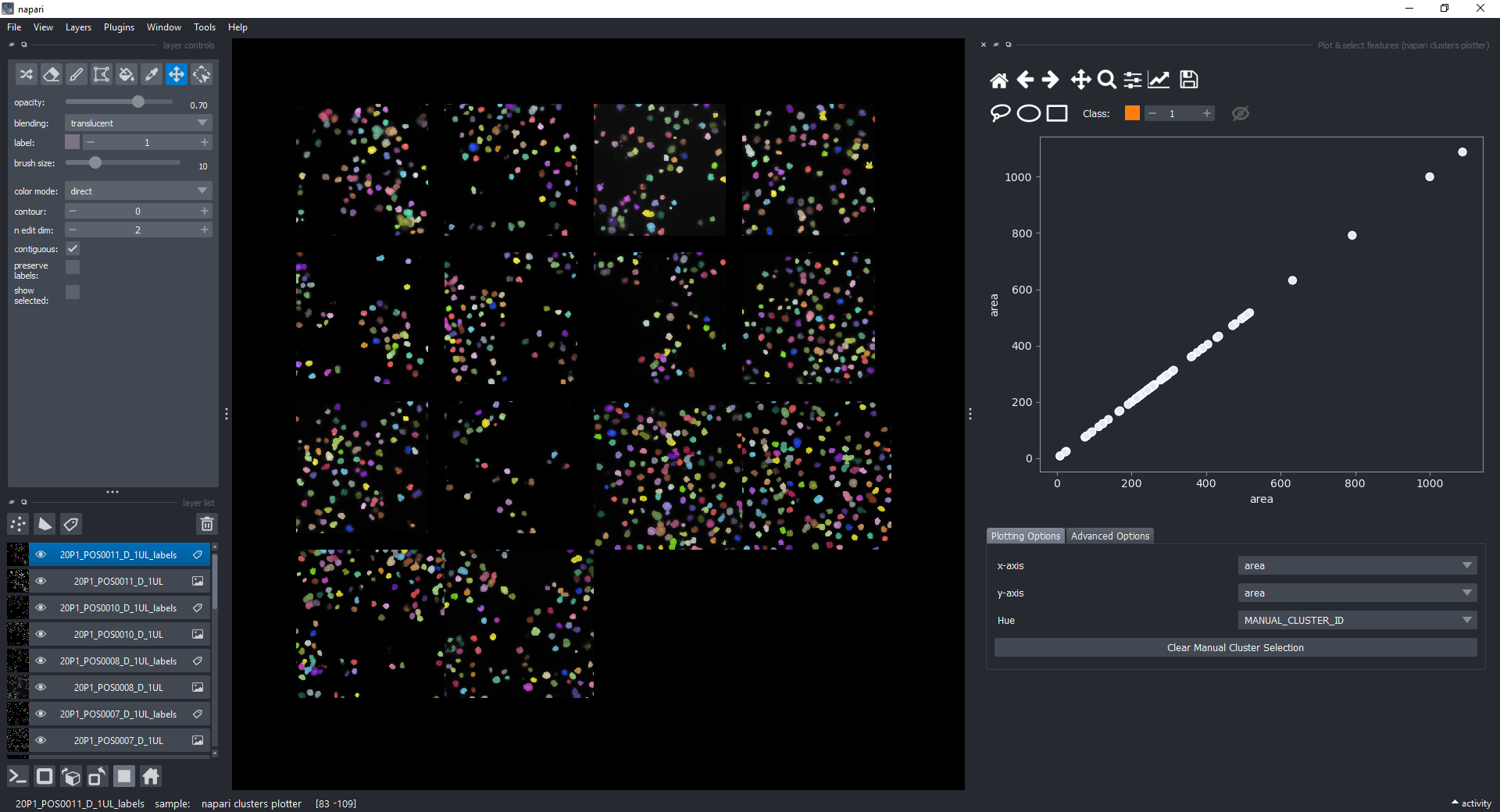
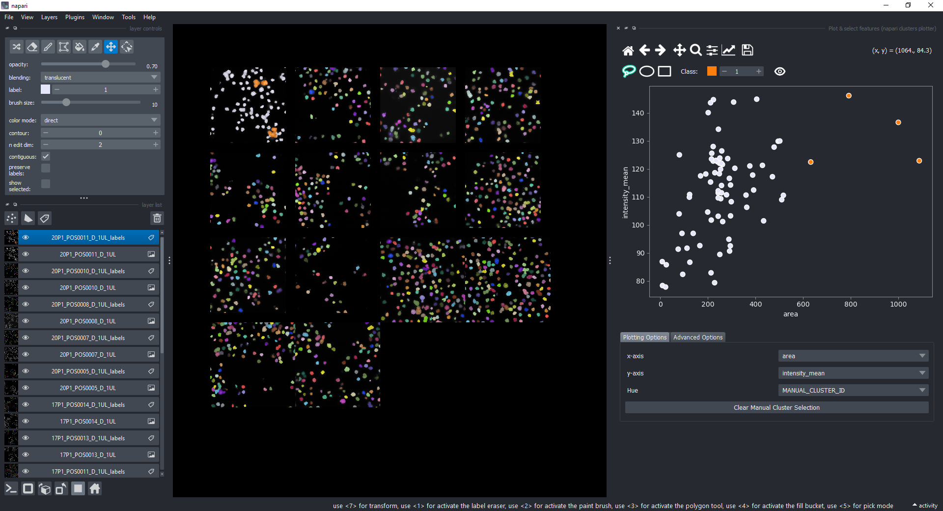
Change the features in the x-axis and y-axis dropdowns (like area and mean_intensity) to have them plotted against each other.

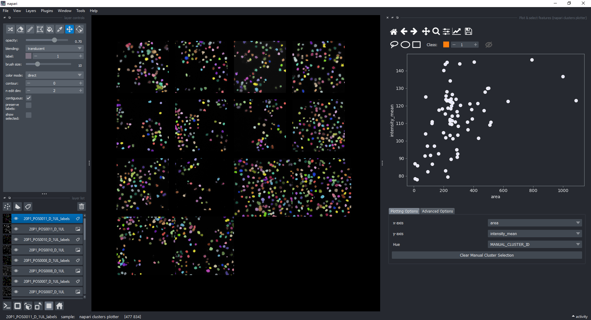
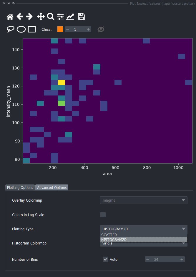
You can explore the Avanced Options tab to change from a scatter plot to a histogram in case there are too many points to visualize.

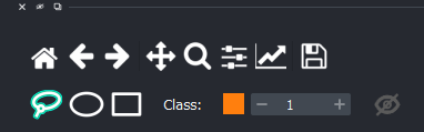
For now, keep the scatter plot and go back to the Plotting Options tab. In the top of the plotter, you can find a few different selector buttons (lasso, ellipse and rectangle), a class spinbox and an eye icon to toggle the visibility of selections/clusters.

Click on the lasso button to have that selector enabled:

Now use the mouse to draw regions around some dots to have the corresponding objects highlighted in the main canvas.

The color of the selected objects in the selected layer (highlighted in blue) will change to the color of the class you have selected in the spinbox. Default is class 1 (orange).

If you now select all the open layers by holding SHIFTand clicking on the first layer and then the last one, you will add features from all layers to the plotter. You can also select individual layers by holding CTRL and clicking on them. If you manually select a region again, you will see that the selected objects in all layers will change to the color of the class you have selected in the spinbox.

Besides manually classifying objects,, you can also change the Hue combobox to map a third feature to the color of the objects in the plotter. For example, you can select eccentricity or perimeter to have the color of the objects in the plotter represent these properties. Notice that categorical features, like the MANUAL_CLUSTER_ID, have their background always highlighted.

Close the plotter.

Dimensionality Reduction

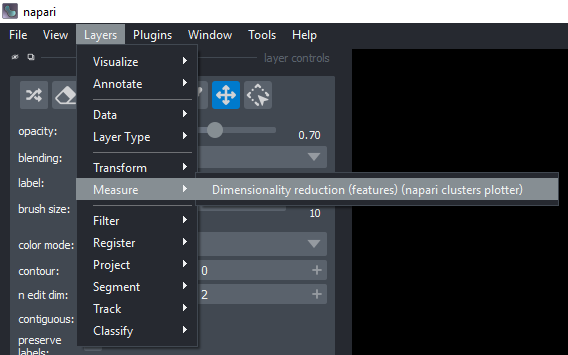
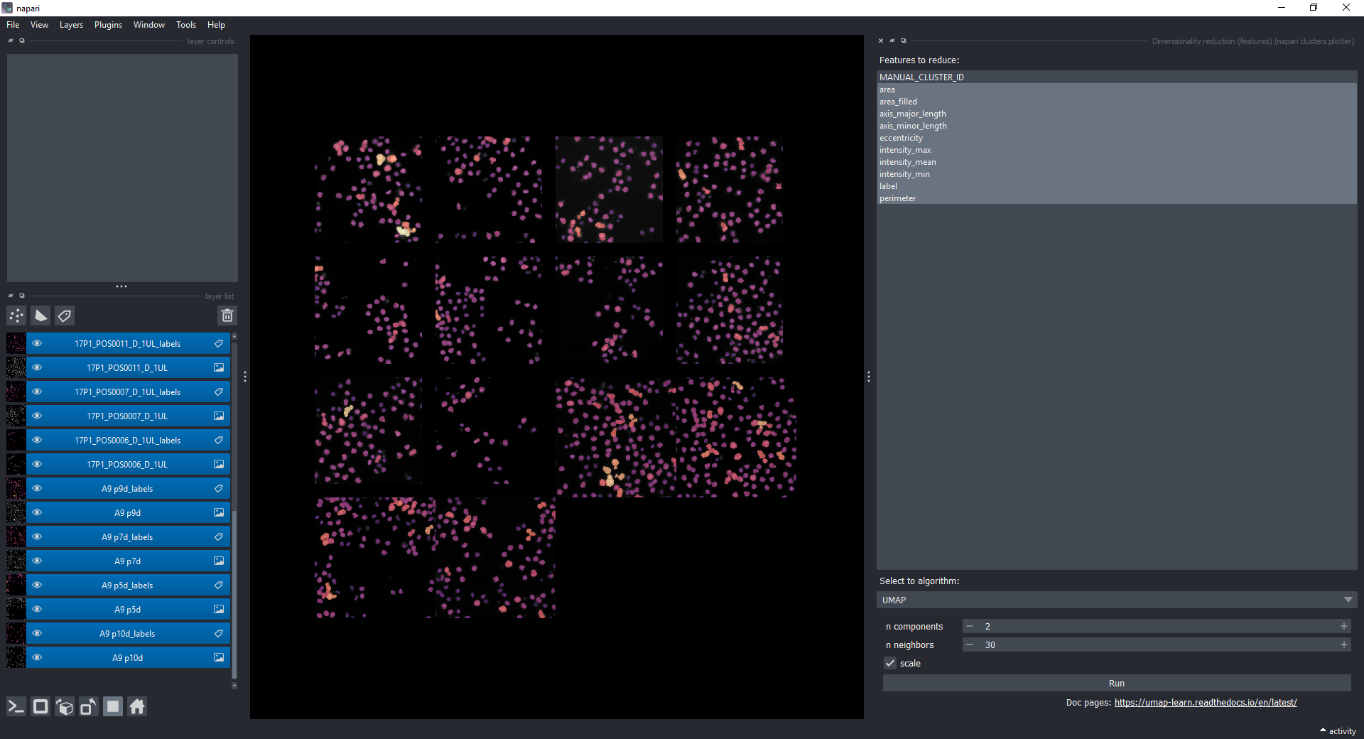
Apply UMAP to have all these dimensions reduced to 2. Do this via Layers > Measure > Dimensionality reduction (features) (napari clusters plotter).

Select all measurements, except MANUAL_CLUSTER_ID (while holding SHIFT, click on the first one, scroll down to the last one and then click on the last one). Choose UMAP under Select algorithm. Make sure to have all layers still selected.

Before you click on Run, notice that there is a small Activity button in the bottom right corner of the napari window. Click on it to open the Activity tab, and now click on Run. You shall see a continuous progress bar in the Activity tab, indicating that the UMAP algorithm is running.

After some time, new columns (UMAP-0 and UMAP-1) will be added to the features. Feel free to close the dimensionality reduction widget.

Visualize Dimensionality Reduction Results

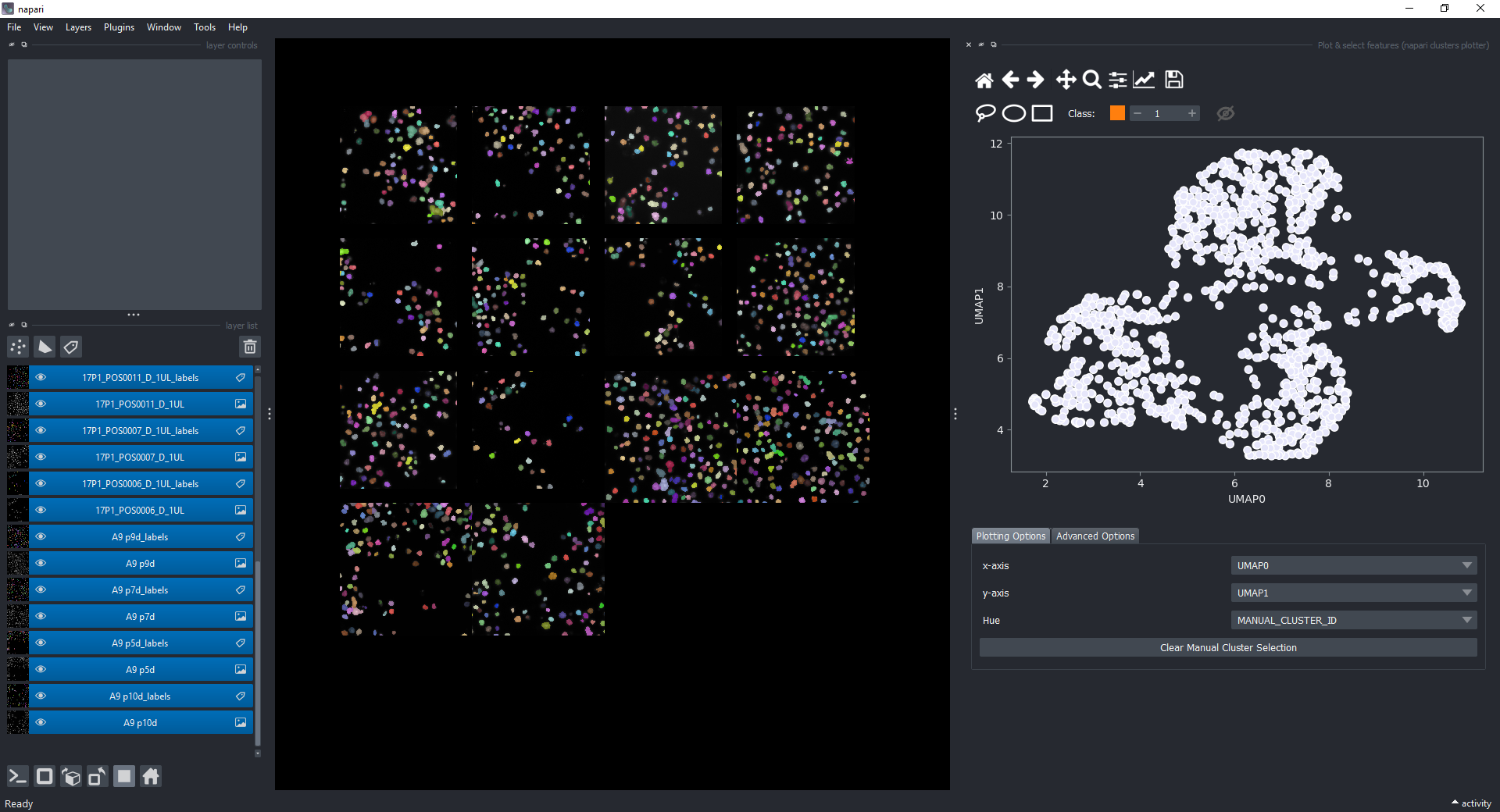
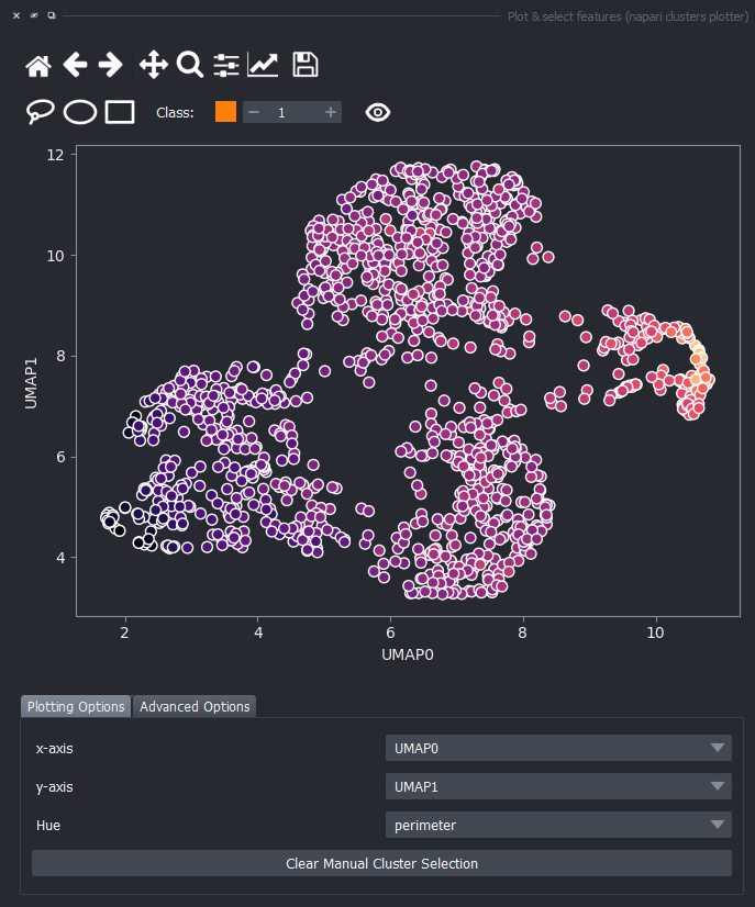
Open the plotter again via Layers > Visualize > Plot & select features (napari clusters plotter) and select UMAP-0 and UMAP-1 in the x-axis and y-axis dropdowns. You should see a plot like this:

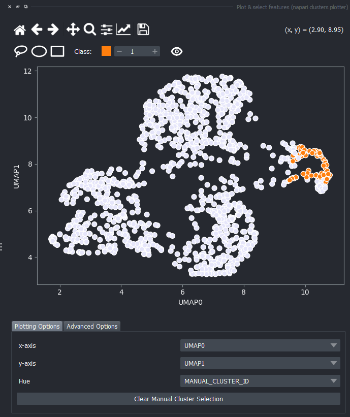
Click on the eye icon to display the previously manual selected objects onto this plot.

You can again change the Hue combobox to visualize a third feature, like perimeter over the UMAP plot.

Clustering

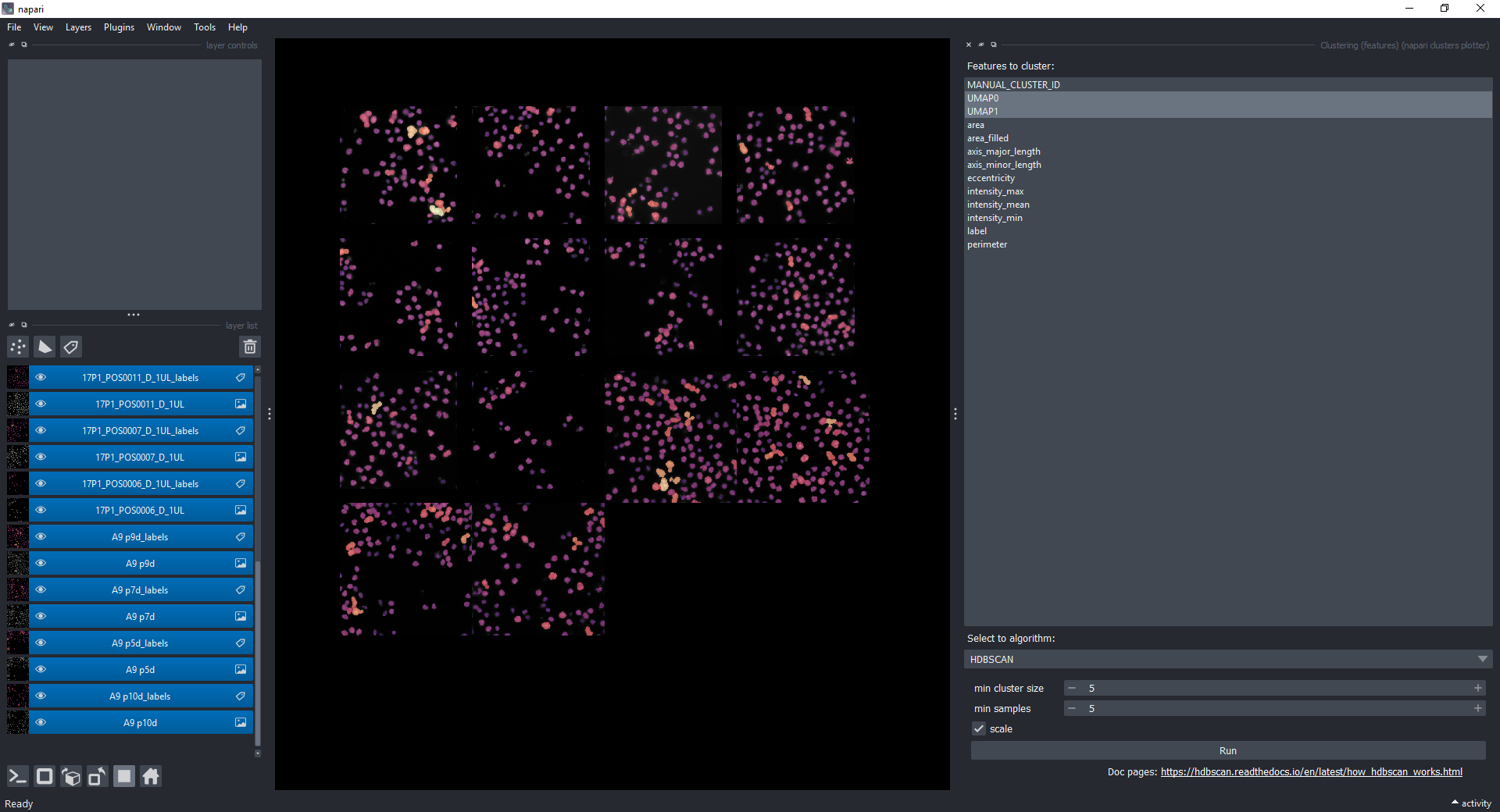
Apply HDBSCAN clustering by first opening the clustering widget via Layers > Classify > Clustering (features) (napari clusters plotter).

Select only UMAP-0 and UMAP-1 now in Measurements (hold CRTL while clicking on them). Under Select algorithm choose HDBSCAN and click on Run.

Visualize Object Classification Results

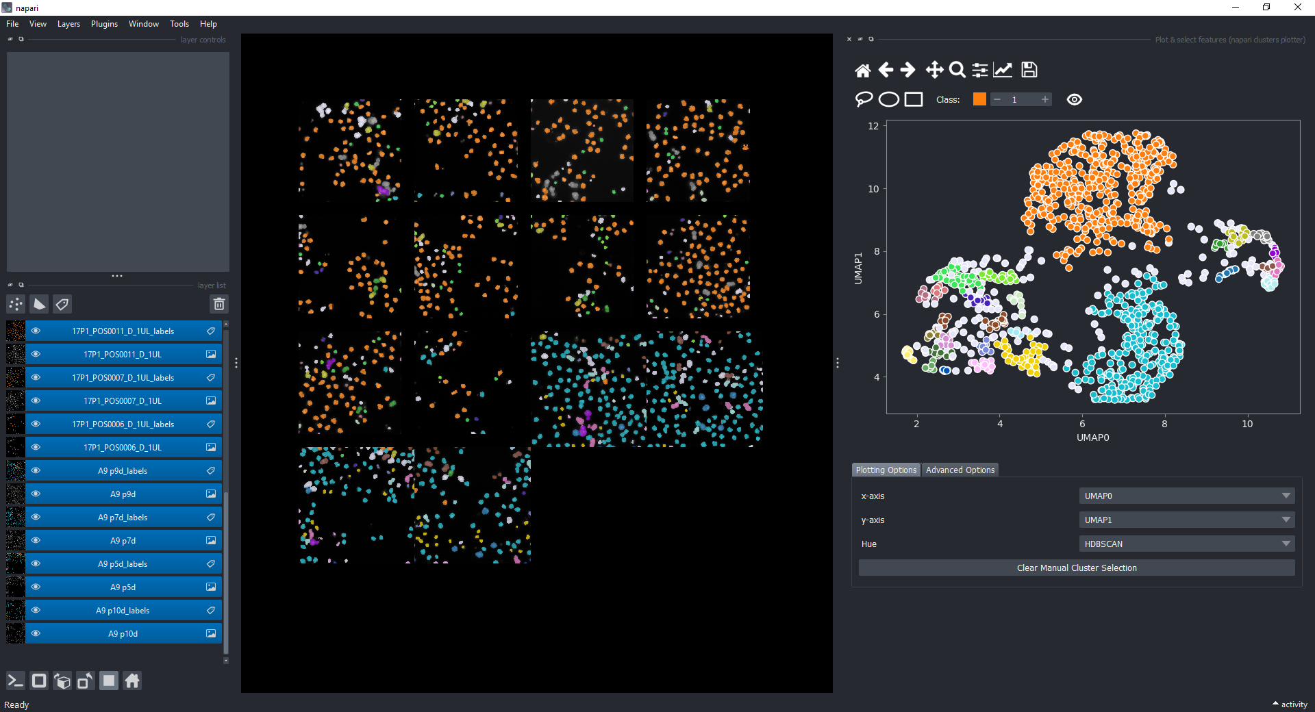
Open the plotter again, plot UMAP-0 and UMAP-1 in the x-axis and y-axis dropdowns, and under Clustering choose HDBSCAN_CLUSTER_ID. You should see a plot like this and the corresponding objects in the napari canvas highlighted in different colors.

Saving the Results

At the moment, you can only display and save individual tables for each Labels layer. This part relies on having napari-tools-menu and napari-skimage-regionprops installed in the environment. To do that, go to Tools > Measurement > Show table (nsr).

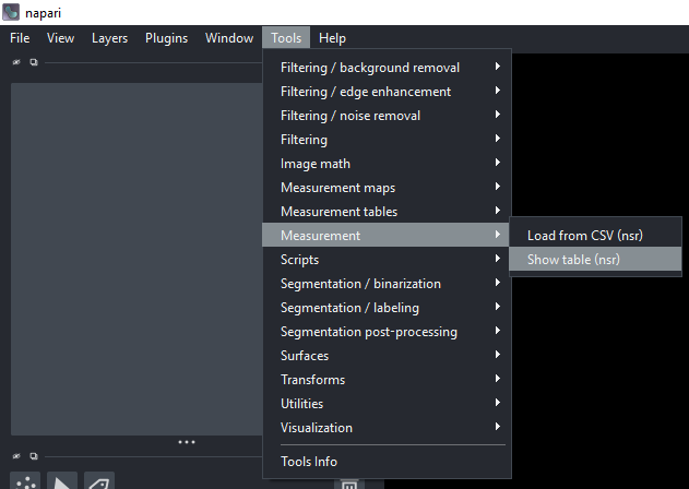
Choose one of the Labels layers and click on Run. You will see a table with all the features for that layer. You can save it as a CSV file by clicking on the Save as csv... button in the top right corner of the table.

Conclusion

Without any ground-truth provided, we just assigned objects to different classes based on some features relationships. We just perfomed an unsupervised machine learning workflow!

Extra Exercise

Explore the other sample datasets in the napari clusters plotter menu. Experiment plotting and classifying:

• Tracks from the TGMM mini dataset,

• Surface vertices with different curvatures from the Cells3D mitotic nucleus surface curvature,

• Shapes representing a skeleton from the skan skeleton dataset.