Interactive unsupervised object classification in Napari

In this exercise we will perfom Feature Extraction, Dimensionality Reduction with UMAP and Clustering with HDBSCAN to assign objects (nuclei) to different classes in napari. We will use the napari plugin napari-clusters-plotter plugin.

Getting started

Open a terminal window and activate your conda environment:

mamba activate napari-intro-env

or

mamba activate devbio-napari

depending which environment you are using.

Afterwards, start up Napari:

napari

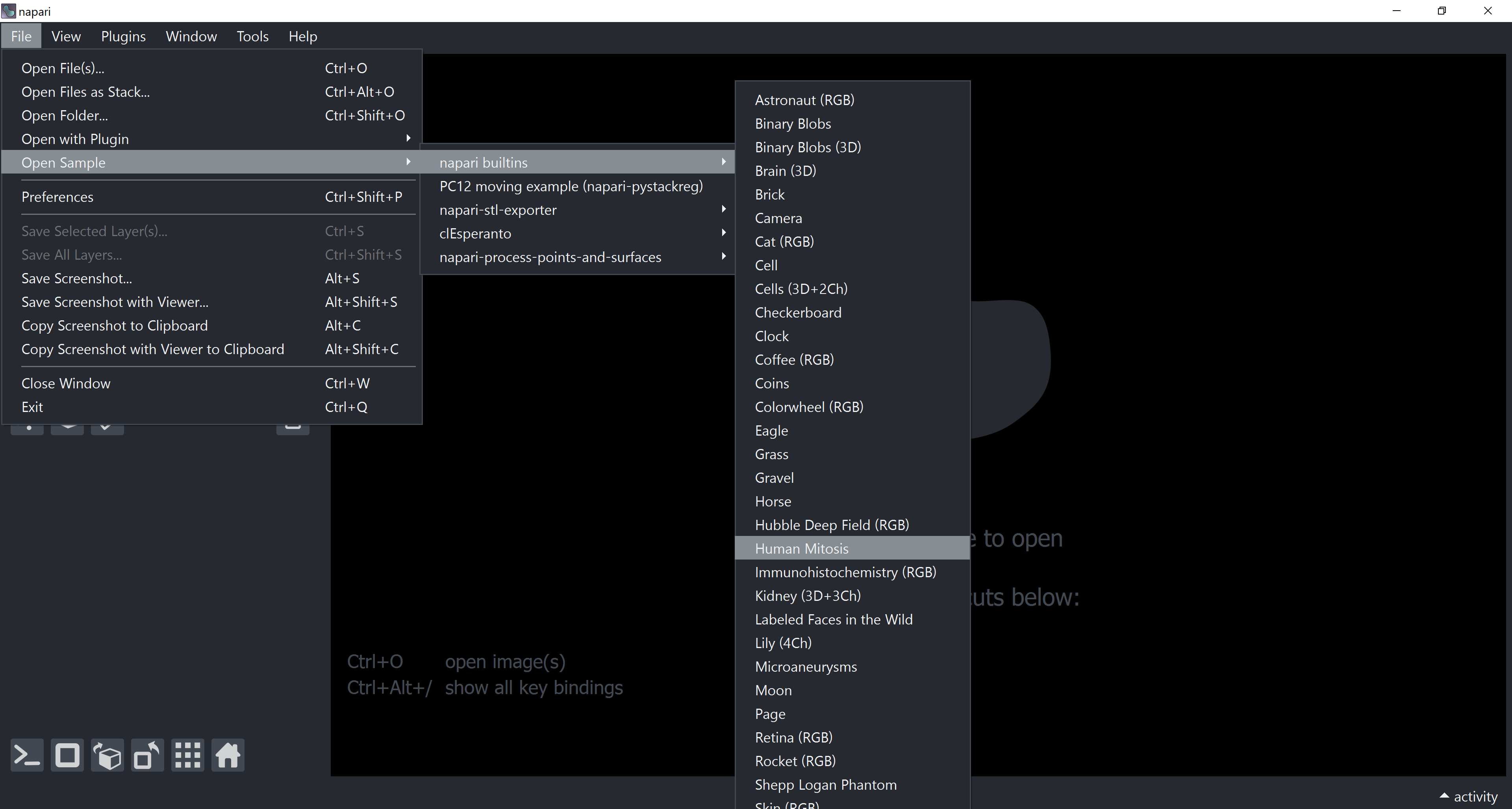
Load the “human-mitosis” example dataset from the menu File > Open Sample > napari builtins > Human Mitosis

Instance Segmentation in Napari

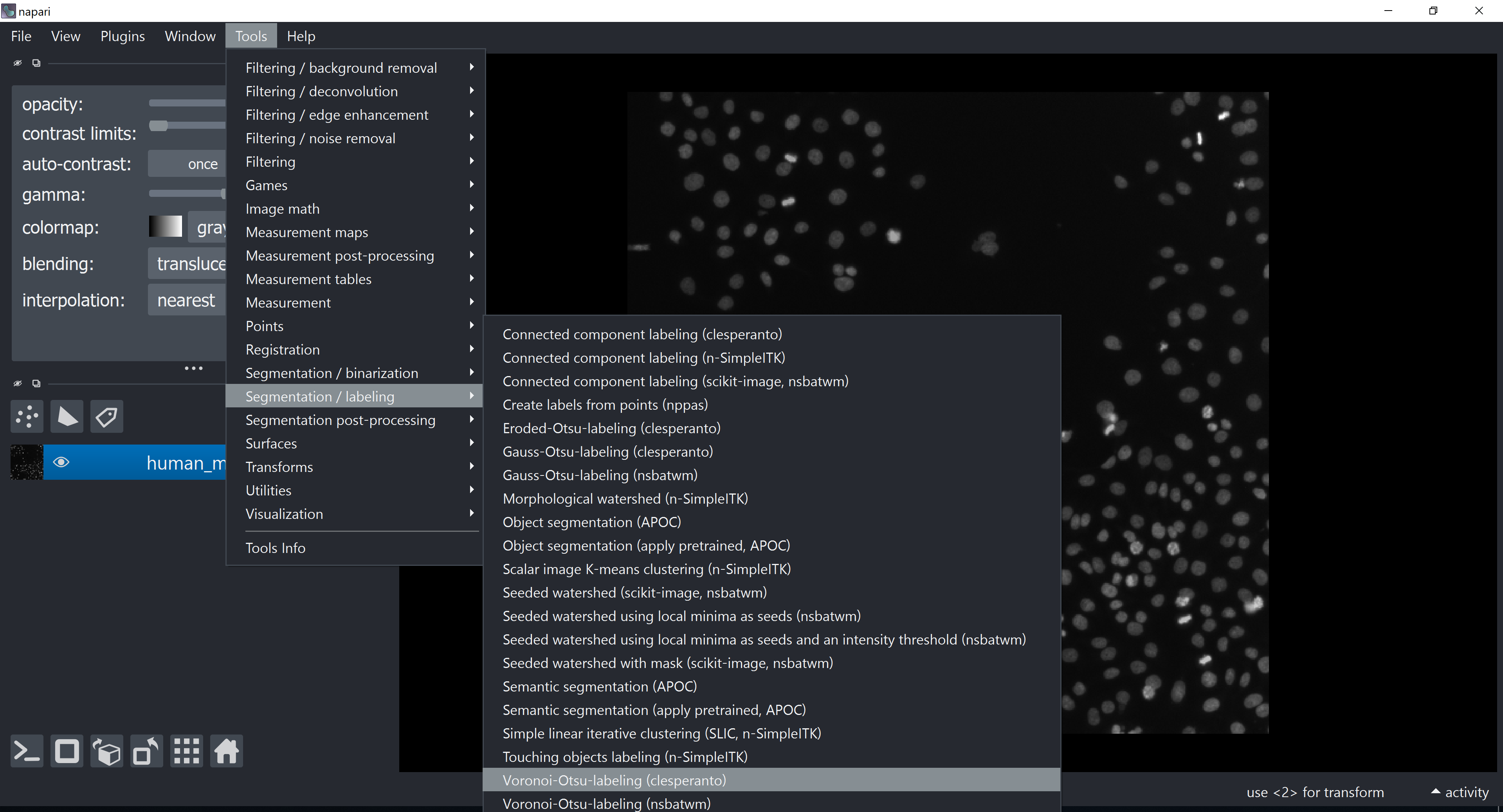
We will first apply the voronoi-otsu-labeling algorithm (from pyclesperanto or nsbatwm) to segment our objects (nuclei). We can do that with through the napari-Assistant plugin or via the Tools menu: Tools > Segmentation / labeling > Voronoi-Otsu-labeling

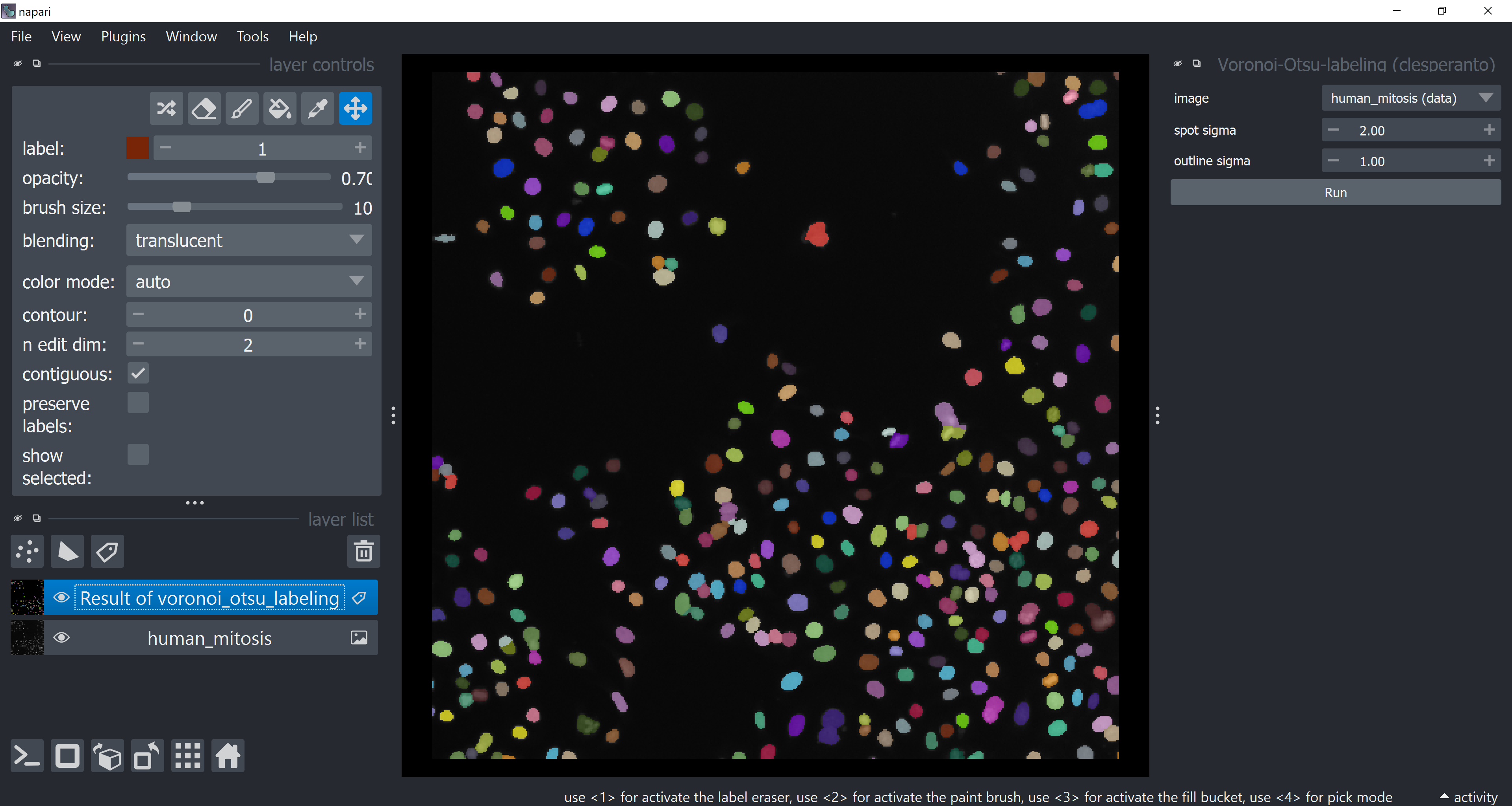
Tune the sigma parameters a bit and click on Run.

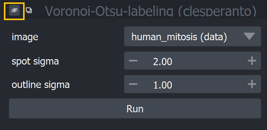
Remember that you can close/hide the widget after having used it so that your screen does not get polluted with lots of open widgets afterwards.

Feature Extraction in Napari

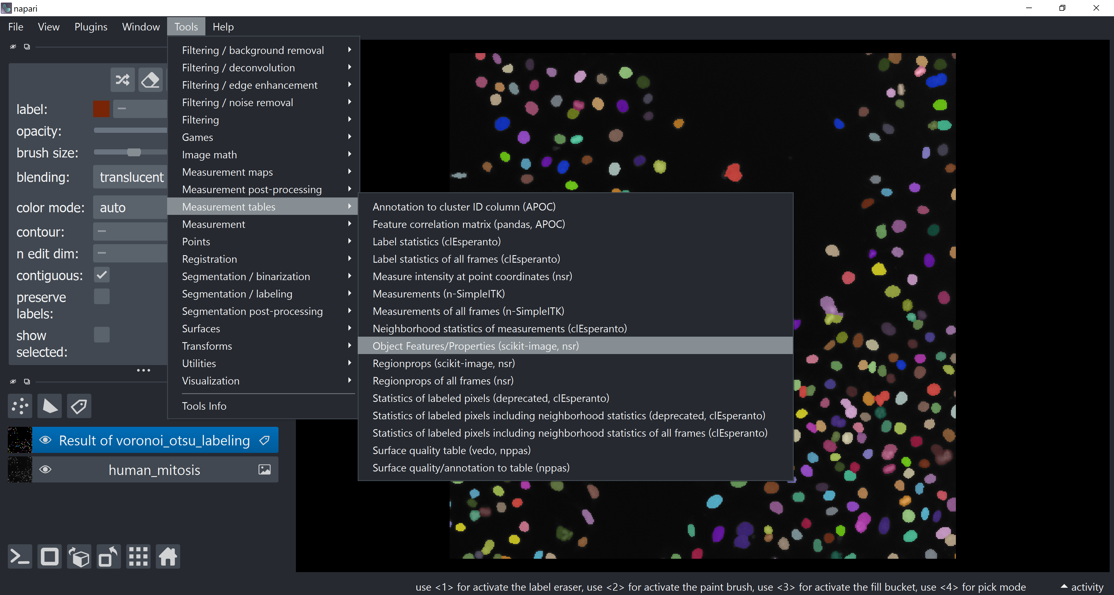
We can extract/calculate lots of object features with the napari-skimage-regionprops plugin. Open the widget via Tools > Measurement tables > Object Features / Properties (scikit-image, nsr).

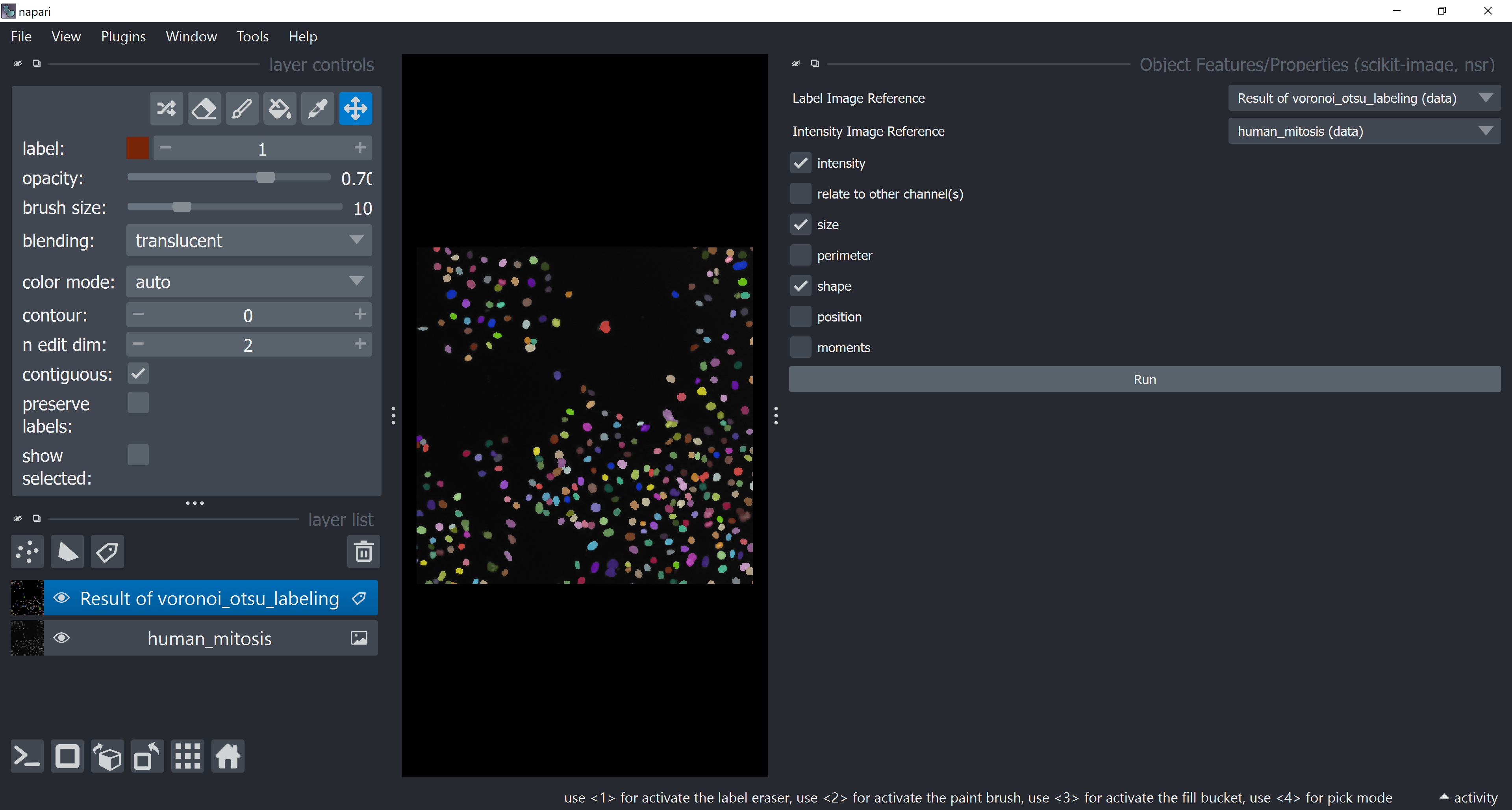
Check intensity, size and shape check boxes and hit the Run button. The Label Image Reference should be the layer with the segmentation results and Intensity Image Reference should be the original human_mitosis image layer from which intensity features will be taken.

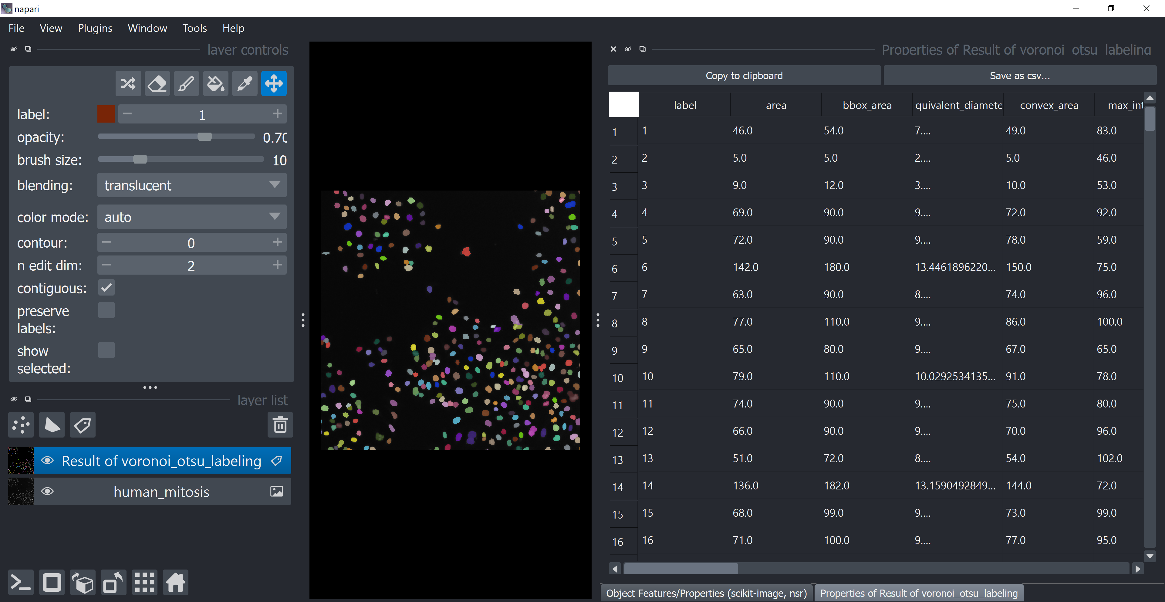
After running it, a table with the features should show up in a different tab (look at the tabs in the lower part of the screen). Feel free to explore it, but consider closing it afterwards for the same reason mentioned before (don’t worry, the table will not get deleted, it is stored within the Labels layer selected at Reference Labels Layer).

Plotting Features in napari

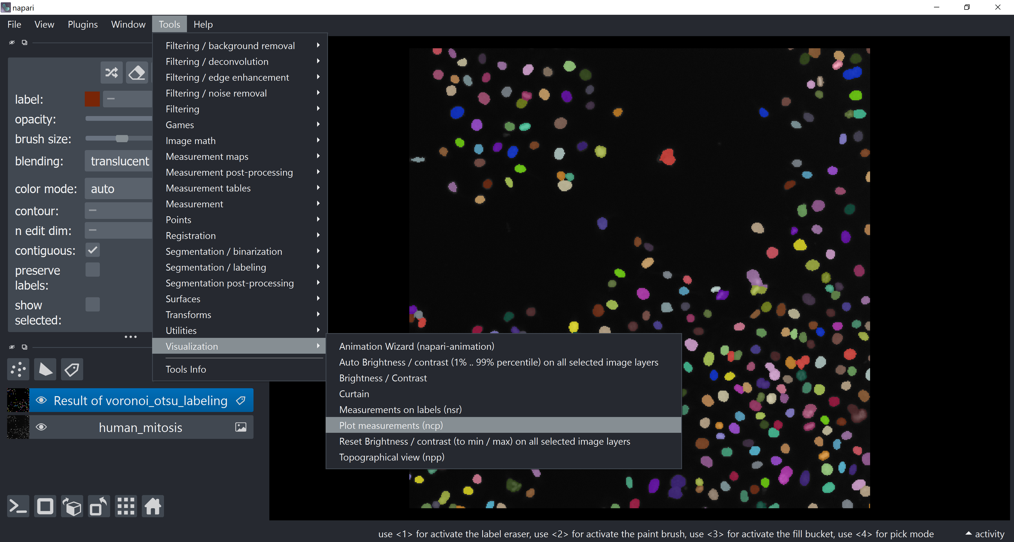
Open the napari-clusters-plotter Plotter via Tools > Visualization > Plot measurements (ncp).

This will open a plotter. Select a few features with the Axes dropdown (like area and mean_intensity) and click on Plot to have them plotted.

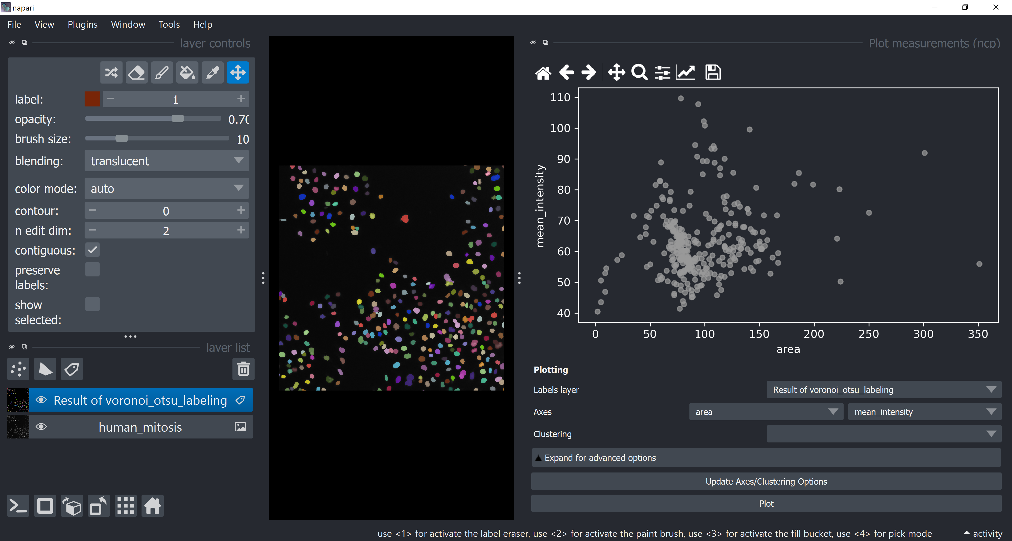
Now use the mouse to draw regions around some dots to have the corresponding objects highlighted in the main canvas as a new Labels layer. Hold SHIFT while dragging the cursor to have new regions with a different color (class).

Close the plotter.

Dimensionality Reduction

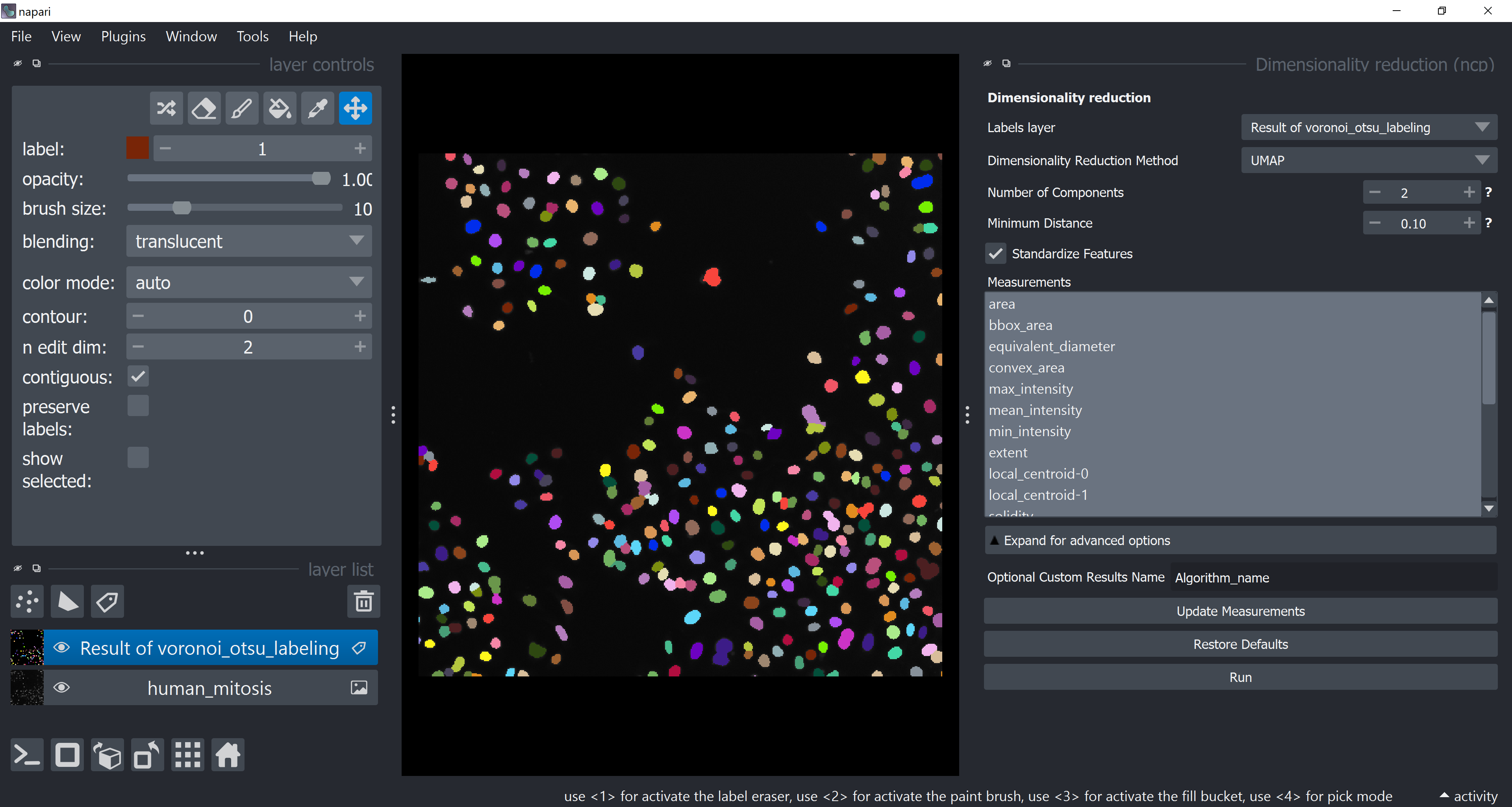
Apply UMAP to have all these dimensions reduced to 2. Do this via Tools > Measurement post-processing > Dimensionality reduction (ncp).

Choose UMAP under Dimensionality Reduction Method. Select all measurements (while holding SHIFT, click on the first one, scroll down to the last one and then click on the last one). Click on Run.

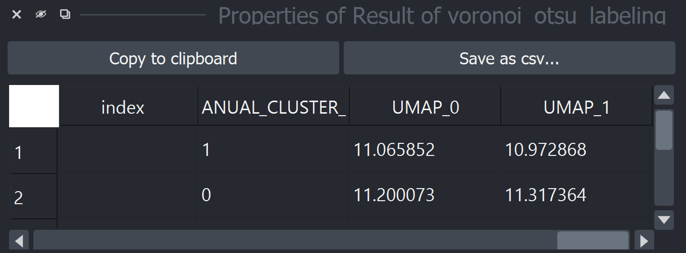
After some time, the table should pop-up again with new columns (UMAP-0 and UMAP-1). Feel free to close the table and the dimensionality reduction widget.

Clustering

Apply HDBSCAN clustering by first opening the clustering widget via Tools > Measurement post-processing > Clustering (ncp). Select only UMAP-0 and UMAP-1 now in Measurements (hold CRTL while clicking on them). Under Clustering Method choose HDBSCAN and click on Run

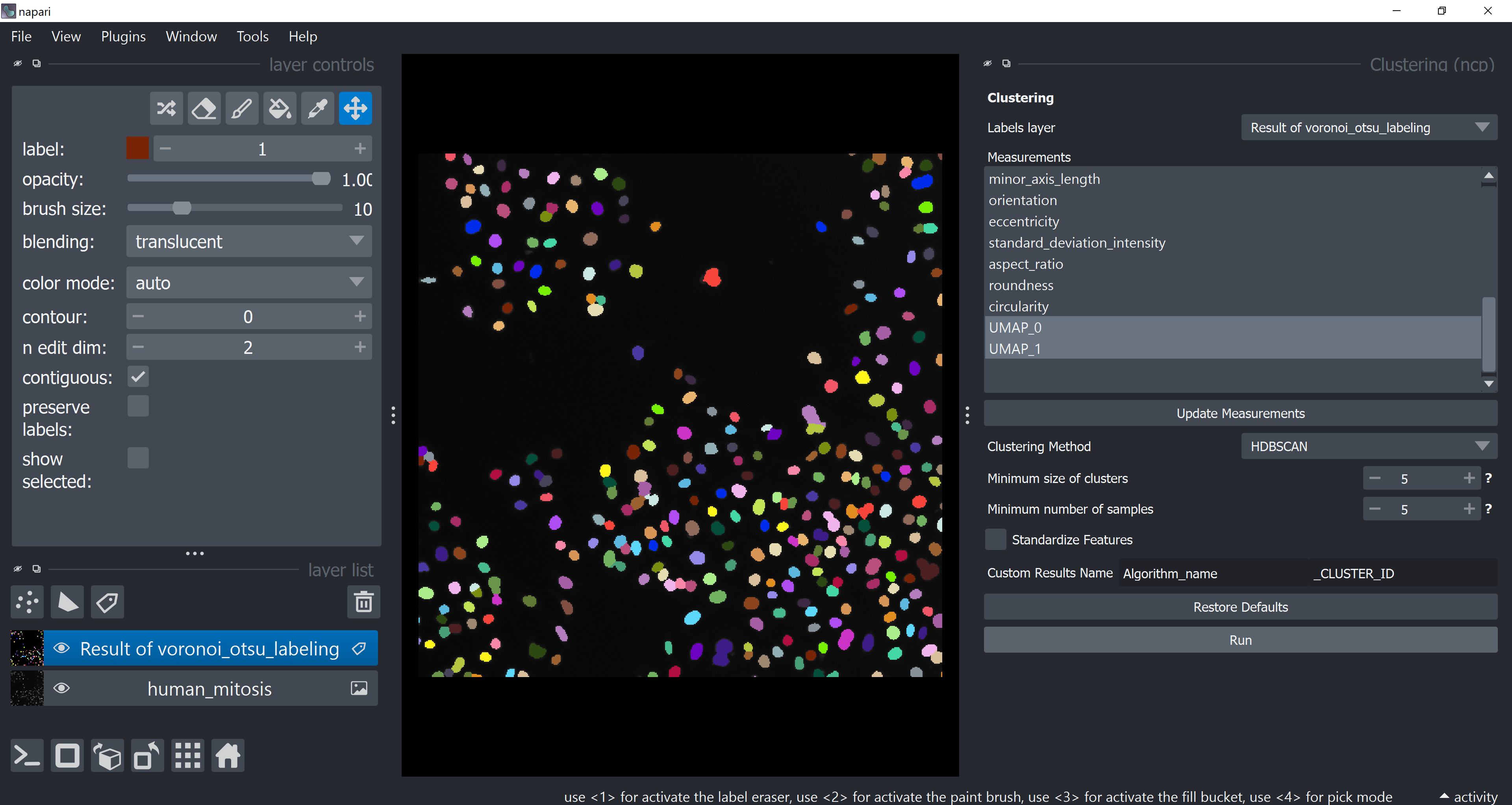
The table should pop-up yet again with a new HDBSCAN_CLUSTER_ID column. Feel free to close it.

Visualize Object Classification Results

Open the plotter again, under Axes choose UMAP-0 and UMAP-1 and under Clustering choose HDBSCAN_CLUSTER_ID. Click on Plot. Try to infer why these classes were classified differently (hide and show layers or turn grid mode on to better inspect results).

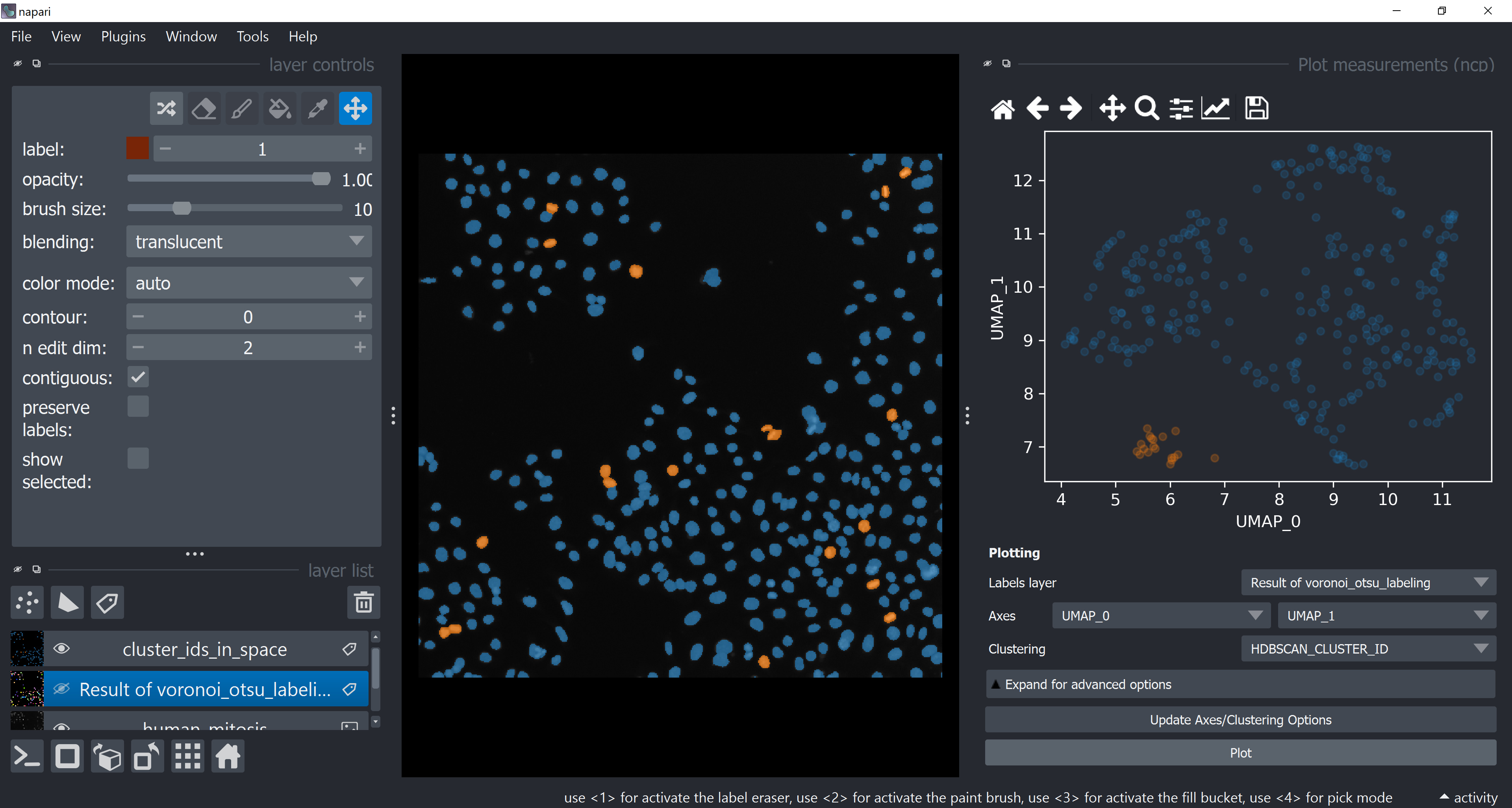
Without any ground-truth provided, we just assigned objects to different classes based on some features relationships. We just perfomed an unsupervised machine learning workflow!